Hypothesis Testing

Hypothesis testing uses statistics to choose between hypotheses regarding whether data is statistically significant or occurred by chance alone. One type of hypothesis tests are t-tests, which are tests that examine whether two means are statistically significantly different from each other or whether the difference between them simply occurred by chance. A One-Sample T-Test compares a sample mean to a known population mean. An Independent Samples T-Test compares two sample means from different populations regarding the same variable. A Paired Samples T-Testcompares two sample means from the same population regarding the same variable at two different times such as during a pre-test and post-test, or it compares two sample means from different populations whose members have been matched. 

One-Sample T-Test

A One-Sample T-Test compares a sample mean and a known population mean to determine whether the difference between the two means is statistically significant or occurred by chance alone.

This example will be comparing the respondents' number of children with the known 2013 United States fertility rate of 2.06 children per woman. The One-Sample T-Test is examining whether the difference between the sample mean number of children per respondent is significantly different from the known population fertility rate.

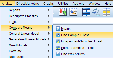
To generate a One-Sample T-Test, click 'Analyze' in the top toolbar of the Data Editor window. Click 'Compare Means' in the dropdown menu, and click 'One-Sample T Test...' in the side menu.

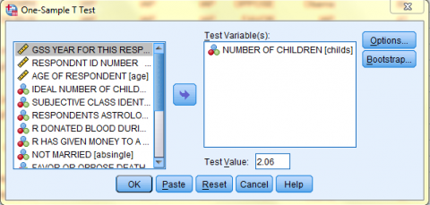
In the One-Sample T Test dialog box that pops up, select the variable of interest (Number of Children, childs) from the list of variables and bring it over to the 'Test Variable(s)' field. Then, enter the known population mean in the 'Test Value:' field. Click 'OK.'

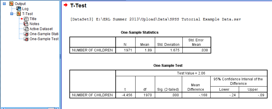
The output is displayed in the SPSS Viewer window. The output consists of two tables. The first table, One-Sample Statistics, contains statistical information about the Number of Children variable, such as N, the Mean, the Standard Deviation, and the Standard Error of the Mean. The second table, One-Sample Test, contains information specific to the One-Sample T-Test, such as the Test Value, the t value, the df (degrees of freedom), the alpha 2-tailed Significance value (when the Sig. value is .05 or less, the probability that the difference between the sample mean and the test value was due to chance is 5% or less), the Mean difference (the difference between the sample mean and the test value), and a 95% Confidence Interval of the Difference. In this case, the difference between the sample mean number of children (1.89) and the known population mean number of children (2.06) is significant.

Independent-Samples T-Test

An Independent-Samples T-Test compares two sample means from different populations regarding the same variable to determine whether the difference between the two means is statistically significant or occurred by chance alone.

This example will be comparing the mean number of hours spent emailing per week (Email Hours Per Week, emailhr) by married respondents and single respondents (Not Married, absingle). The 'Email Hours Per Week, emailhr' variable is the test variable, and the 'Not Married, absingle' variable is the nominal grouping variable. The Independent-Samples T-Test is examining whether the difference between the mean number of hours married respondents spent emailing and the mean number of hours single respondents spent emailing is significantly different or occurred by chance.

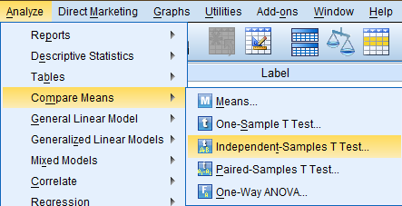
To generate a Independent-Samples T-Test, click 'Analyze' in the top toolbar of the Data Editor window. Click 'Compare Means' in the dropdown menu, and click 'Independent-Samples T Test...' in the side menu.

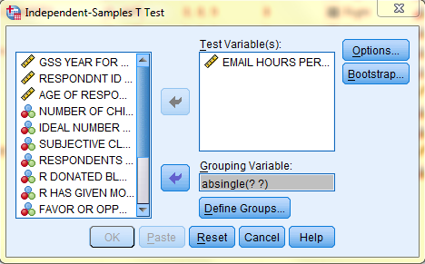
In the Independent-Samples T Test dialog box that pops up, select the variable of interest (Email Hours Per Week, emailhr) from the list of variables and bring it over to the 'Test Variable(s)' field. Then, enter the nominal grouping variable (Not Married, absingle) in the 'Grouping Variable:' field. Then click 'Define Groups...' to identify the two populations being compared.

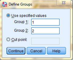
In the Define Groups dialog box, select 'Use specifiec values' and enter the Value Labels of the nominal grouped variable. In this example, Group 1 will correspond with Value Label 1, which refers to the respondents who indicated they are not married ('Yes'), and Group 2 will correspond with Value Label 2, which refers to the respondents who indicated they are married ('No'). Then, click 'Continue,' and back in the Independent-Samples T Test dialog box, click OK.

The output is displayed in the SPSS Viewer window. The output consists of two tables. The first table, Group Statistics, contains statistical information about the Email Hours Per Week variable, split by whether the respondent is not married (indicated in the chart by Yes) or is married (indicated in the chart by No). For each group of respondents, the N, the Mean, the Standard Deviation, and the Standard Error of the Mean are displayed.

The second table, Independent-Samples Test, contains information specific to the Independent-Samples T-Test, such as information about Levene’s Test for Equality of Variances and the t-test for Equality of Means. Levene’s Test for Equality of Variances tests whether variability within each group (married or not married) is equal. The outputs displays two sets of results: one set in which equal variance is assumed and one set in which equal variance is not assumed. It is up to the user to determine which set of results is appropriate. You can determine which results are appropriate by looking at the Sig., the alpha level of significance. If the alpha level is greater than .05, then group variances are assumed to be equal. In this example, Sig. is greater than .05 so group variances are assumed to be equal, and we read the top line of the table. The portion of the table dedicated to the t test for Equality of Means displays the t value, the df (degrees of freedom), the 2-tailed Sig. value (when the Sig. value is .05 or less, the probability that the difference between the two means was due to chance is 5% or less), the Mean difference (the difference between the two means), and a 95% Confidence Interval of the Difference. In this case, the difference between the two means is not significant and could have occured by chance.

Paired Samples T-Test

A Paired Samples T-Test compares two sample means from the same population regarding the same variable at two different times such as during a pre-test and post-test, or it compares two sample means from different populations whose members have been matched, to determine whether the difference between the two means is statistically significant or occurred by chance alone.

This example will be comparing the respondents' mean number of children (Number of Children, childs) with the respondents' mean ideal number of children (Ideal Number of Children, chldidel). The respondents in this example are paired with themselves. The Paired-Samples T-Test is examining whether the difference between the mean number of children and the mean ideal number of children is significantly different or occurred by chance.

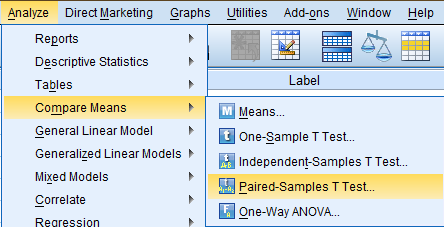
To generate a Paired-Samples T-Test, click 'Analyze' in the top toolbar of the Data Editor window. Click 'Compare Means' in the dropdown menu, and click 'Paired-Samples T Test...' in the side menu.

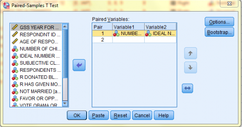
In the Paired-Samples T Test dialog box that pops up, select the variables of interest (Number of Children, childs, and Ideal Number of Children, chldidel) from the list of variables and bring them over to the 'Paired Variables:' field. Then, click 'OK.'

The output is displayed in the SPSS Viewer window. The output consists of three tables. The first table, Paired Samples Statistics, contains statistical information about the Number of Children and Ideal Number of Children variables. For each variable, the Mean, the N, the Standard Deviation, and the Standard Error of the Mean are displayed. The second table, Paired Samples Correlations, contains a correlation value measuring how closely related the two variables are to each other. The correlation value is the correlation coefficient of the two variables and measures the strength and direction of the linear relationship between the two variables. Specifically, the closer the correlation value to 1 or -1, the more strongly linearly related the variables. In this example, the correlation value is not close to 1 so the variables do not have a strong linear relationship.

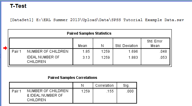
The third table, Paired Samples Test, displays the Mean (referring to the difference between the two means), the Standard Deviation of the Mean, the Standard Error of the Mean, and a 95% Confidence Interval of the Difference. The table also displays the t value, the df (degrees of freedom), and the 2-tailed Sig. value (when the Sig. value is .05 or less, the probability that the difference between the two means was due to chance is 5% or less). In this case, the difference between the two means is significant.

Hypothesis Testing uses statistics to choose between hypotheses regarding whether data is statistically significant or occurred by chance alone. One type of hypothesis tests are ANOVA tests, which are tests that examine whether two or more means are statistically significantly different from each other or whether the difference between them simply occurred by chance. ANOVA stands for Analysis of Variance. A One-Way ANOVA compares the means of two or more groups. A Factorial ANOVA compares the means of two or more groups while examining the interaction of and between two independent variables. (However, the ANOVA tests do not specify which groups differ significantly, and since there are more than two groups, in order to determine which groups differ, further statistical analyses and Post Hoc tests must be done and can be added to the ANOVA procedure in SPSS.)

One-Way ANOVA

A One-Way ANOVA compares the means of two or more groups. A One-Way ANOVA thus requires one categorical variable consisting of two or more groups, serving as the independent variable, and one continuous variable, serving as the dependent variable.

In this example, the variable 'Subjective Class Identification, class' will be serving as the categorical variable with 4 groups, and the variable 'Number of College-Level Sci Courses R Have Taken, colscinm' will be serving as the continuous variable. The One-Way ANOVA is specifically looking at whether respondents of different subjective class identifications differ significantly in the mean number of college-level science classes taken.

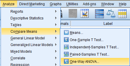
To generate a One-Way ANOVA, click 'Analyze' in the top toolbar of the Data Editor window. Click 'Compare Means' in the dropdown menu, and click 'One-Way ANOVA...' in the side menu.

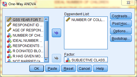
In the One-Way ANOVA dialog box that pops up, select the dependent variable of interest (Number of College-Level Sci Courses R Have Taken, colscinm) from the list of variables and bring it over to the 'Dependent List:' field. Then, select the nominal grouping variable of interest (Subjective Class Identification, class) from the list of variables and bring it over to the 'Factor' field. To include Post Hoc tests in the ANOVA output, click 'Post Hoc...'

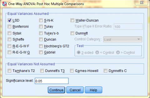
In the One-Way ANOVA: Post Hoc Multiple Comparisons dialog box that pops up, select the desired Post Hoc test. In this example, we will be using Least Significant Difference (LSD) tests. Then, click 'Continue.'

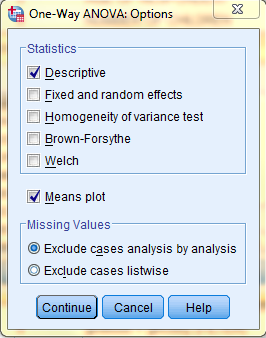
Back in the One-Way ANOVA dialog box, click 'Options' if you would like to add any other statistics to the ANOVA output. Here, we selected to include a Descriptives table and a Means plot in the output. Click 'Continue.' Then, back in the One-Way ANOVA dialog box, click 'OK.'

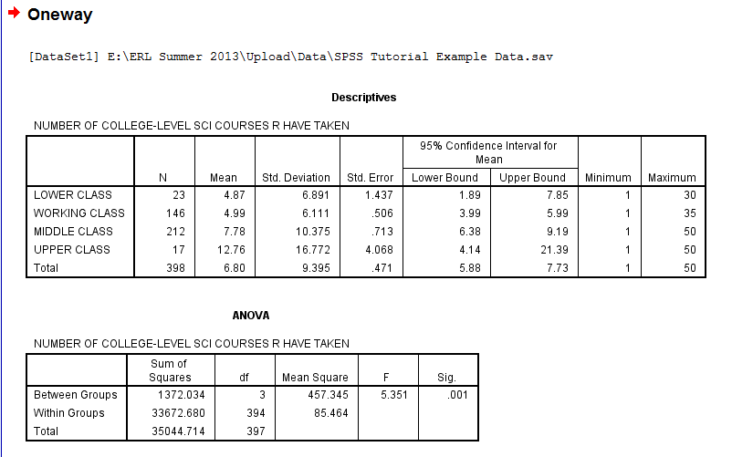
The output is displayed in the SPSS Viewer window. The output consists of four parts. The first table, Descriptives, contains statistical information about the dependent variable, Number of College-Level Sci Courses R Have Taken, split by the independent variable groupings, the respondents' Subjective Class Identification. For each group of respondents, the N, the Mean, the Standard Deviation, the Standard Error of the Mean, a 95% confidence Interval for the Mean, the Minimum value, and the Maximum value are displayed. The second table, ANOVA, contains information about the ANOVA test comparing means both between and within groups and includes the Sum of Squares (a measure of variance), df (degrees of freedom), Mean Square, the F value, and the Sig. value (when the Sig. value is .05 or less, the probability that the difference between the groups was due to chance is 5% or less). In this case, some of the means are significantly different from each other. However, the results of the ANOVA alone do not indicate which groups differ significantly. Thus, the Multiple Comparisons Output which displays the results of the Post Hoc LSD test is necessary.

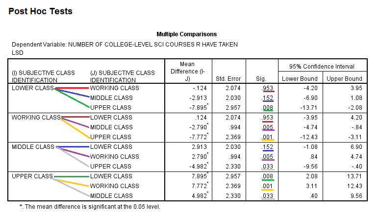
The next table, Multiple Comparisons Output, displays the results of the LSD test. The LSD test compares each group (class category) to all other groups (class categories). Thus, please note that this table displays some comparisons more than once, since, in every row, each group is compared to all other groups. Each comparison is denoted by a differnet color, and lines of the same color represent repeated comparisons. For each comparison, the table displays the Mean Difference (the difference between the groups' mean number of college-level science classes taken), the Standard Error, the Sig. value (when the Sig. value is .05 or less, the probability that the difference between the groups was due to chance is 5% or less), and a 95% Confidence Interval for the Mean Difference. In this example, the Upper Class differs significantly from the Lower, Working, and Middle Classes, and the Middle Class differs significantly from the Working Class in the number of college-level science courses taken.

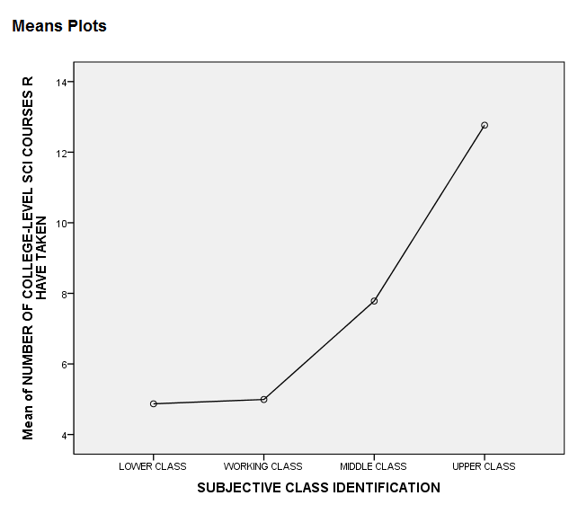
The last section of the output, the Means Plot, is a graphical display of how the mean number of college-level science courses the respondents have taken depends on subjective class identification.

Factorial ANOVA

A Factorial ANOVA compares the means of two or more groups while examining the interaction of and between two independent variables. A Factorial ANOVA thus requires one continuous variable to serve as the dependent variable and more than one categorical variable (each consisting of two or more groups) to serve as the independent variables.

In this example, the variable 'Subjective Class Identification, class' will be serving as the first categorical variable with 4 groups, and the variable 'Not Married, absingle' will be serving as the second categorical variable with 2 groups. The variable 'Hours Per Day Watching TV, tvhours' will serve as the continuous variable. The Factorial ANOVA is specifically looking at whether respondents of different subjective class identifications and of different marital statuses differ significantly in the mean number hours spent watching tv per day.

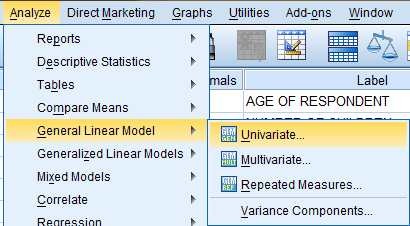
To generate a Factorial ANOVA, click 'Analyze' in the top toolbar of the Data Editor window. Click 'General Linear Model' in the dropdown menu, and click 'Univariate...' in the side menu.

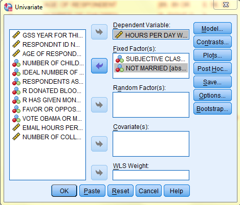
In the Univariate dialog box that pops up, select the dependent variable of interest (Hours Per Day Watching TV, tvhours) from the list of variables and bring it over to the 'Dependent Variable:' field. Then, select the nominal independent grouping variables of interest (Subjective Class Identification, class, and Not Married, absingle) from the list of variables and bring them over to the 'Fixed Factor(s):' field. To include Post Hoc tests in the ANOVA output, click 'Post Hoc...'

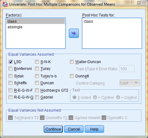
In the Univariate: Post Hoc Multiple Comparisons for Observed Means dialog box that pops up, select the desired variable for which you wish to run a Post Hoc Test (any variable with more than two groups, which, in this case, is the 'class' variable). In this example, we will be using Least Significant Difference (LSD) tests. Then, click 'Continue.'

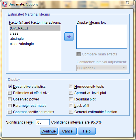
Back in the Univariate dialog box, click 'Options' if you would like to add any other statistics to the ANOVA output. Here, we selected to include a Descriptives table in the output. Click 'Continue.' Then, back in the One-Way ANOVA dialog box, click 'OK.'

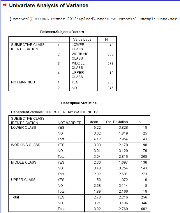
The output is displayed in the SPSS Viewer window. The output consists of four parts. The first table, Between-Subjects Factors, lists the independent variables Value Labels and N, the group size, for each group. The second table, Descriptive Statistics, contains statistical information about the dependent variable, Hours Per Day Watching TV, displayed corresponding with each of the indepedent variable groups: the respondents' Subjective Class Identification and marital status. For each group of respondents, the Mean, the Standard Deviation, and the N are displayed.

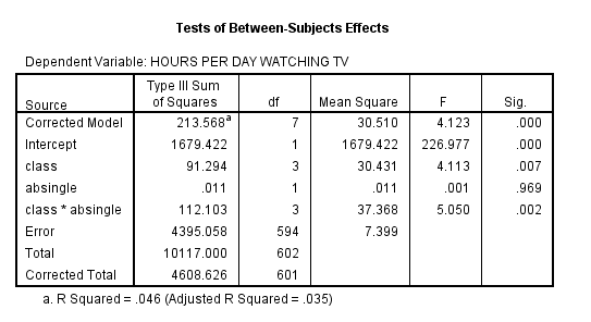
The third table, Tests of Between-Subjects Effects, contains information about the Factorial ANOVA test and includes the Sum of Squares (a measure of variance), df (degrees of freedom), Mean Square, the F value, and the Sig. (when the Sig. value is .05 or less, the probability that the difference between the means was due to chance is 5% or less). The first two rows of the table, Corrected Model and Intercept are advanced statistics and will not be addressed in this tutorial. The next rows correspond with the independent variables, and their significance levels are measured separately, demonstrating the influence of each independent variable individually on the number of hours per day spent watching TV. There is also a row showing the interaction between the two independent variables, demonstrating whether the two independent variables interacted to significantly impact the results. In this case, class influenced the number of hours respondents spent watching TV but marital status did not. Additionally, there was a significant interaction between class and marital status.

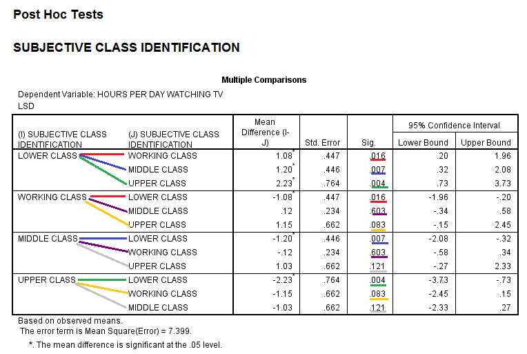
The next table, Multiple Comparisons, displays the results of the LSD test. The results of the ANOVA alone did not indicate which class groups differ significantly. Thus, the Multiple Comparisons table, which displays the results of the Post Hoc LSD test, is necessary. The LSD test compares each group (class category) to all other groups (class categories). Thus, please note that this table displays some comparisons more than once, since, in every row, each group is compared to all other groups. Each comparison is denoted by a differnet color, and lines of the same color represent repeated comparisons. For each comparison, the table displays the Mean Difference (the difference between the groups' mean number of hours spent watching TV), the Standard Error, the Sig. value (when the Sig. value is .05 or less, the probability that the difference between the means was due to chance is 5% or less), and a 95% Confidence Interval for the Mean Difference. In this example, the Lower Class differs significantly from the Working, Middle, and Upper Classes in the amount of time spent watching TV per day.

Hypothesis Testing uses statistics to choose between hypotheses regarding whether data is statistically significant or occurred by chance alone. One type of hypothesis tests are Chi-Square tests, which are tests that examine whether the frequency of certain categorical values, such as the number of individuals in a group, differs from the frequency distribution expected from random chance alone. The Chi-Square Goodness of Fit Test does this for one variable at a time, and the Test of Independence: Pearson's Chi-Square does this as well but can also test whether multiple categorical variables are significantly associated.

Goodness of Fit Test

A Chi-Square Goodness of Fit Test examines whether the frequency of certain categorical values differs from the frequency distribution expected from random chance alone. The Chi-Square Goodness of Fit Test does this for one variable at a time and requires a categorical variable consisting of two or more groups as input.

In this example, the variable 'Respondents Astrological Sign, zodiac' will be serving as the categorical variable with 12 groups. The Chi-Square Goodness of Fit Test is specifically looking at whether the respondents' astrological signs differ significantly in distribution from one that is expected by random chance. (This example is operating under the assumption that the frequency distribution expected from random chance alone should have all of the categories equally represented with an equal number of people with each zodiac.)

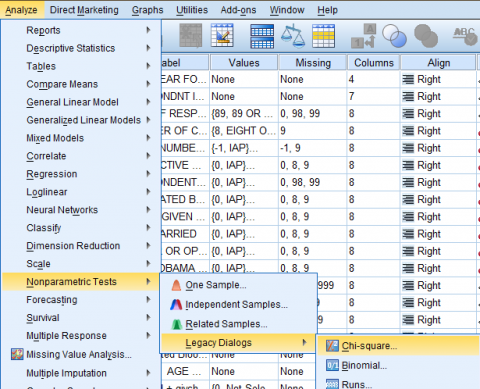
To generate a Chi-Square Goodness of Fit Test, click 'Analyze' in the top toolbar of the Data Editor window. Click 'Nonparametric Tests' in the dropdown menu, and click 'Legacy Dialogs...' in the first side menu and 'Chi Square' in the second side menu.

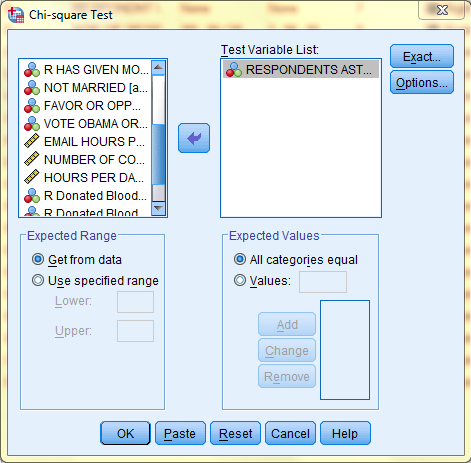
In the Chi Square dialog box that pops up, select the variable of interest (Respondents Astrological Sign, zodiac) from the list of variables and bring it over to the 'Test Variable List:' field. Then, in the 'Expected Values' field, select 'All categories equal' if all groups would be expected to have equal frequencies, or enter an exact value if a specific frequency is expected. In this case, we selected 'All categories equal' because we are operating under the assumption that the frequency distribution expected from random chance alone should have all of the categories equally represented with an equal number of people with each zodiac. Then, click 'OK.'

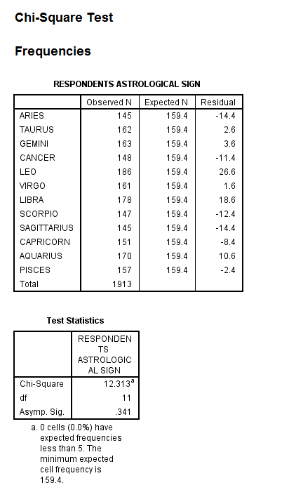
The output is displayed in the SPSS Viewer window. The output consists of two tables. The first table, Respondents Astrological Sign, displays the Observed N, the Expected N, and the Residual (the difference between the Observed N and the Expected N) for each of the categories within the categorical variable (for each of the astrological signs). The second table, Test Statistics, displays information specific to the Chi-Square Goodness of Fit Test, including the Chi-Square Value, the df (degrees of freedom), and Asymp. Sig. (when the Sig. value is .05 or less, the probability that the difference between the Observed N and Expected N value was due to chance is 5% or less). In this case, the Sig. level is above .05, so the difference between the Observed and Expected N values is not significant and the sample is an accurate representation of the population.

Test of Independence: Pearson's Chi-Square

Test of Independence: Pearson's Chi Square examines whether the frequency of certain categorical values differs from the frequency distribution expected from random chance alone. The Test of Independence: Pearson's Chi Square does this for one variable at a time but it also tests whether the multiple categorical variables are significantly associated. It requires two categorical variables consisting of two or more groups as input, .

In this example, the variable 'Subjective Class Identification, class' with 4 groups, and the variable 'R Has Given Money To A Charity, givchrty' with 6 groups will be serving as the categorical variables. The Test of Independence: Pearson's Chi Square is specifically looking at whether the two variables are significantly associated, with the distribution of the respondents' subjective class identification and frequency of giving money to a charity differing from the distribution expected by random chance.

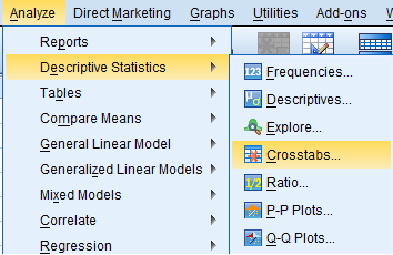
To generate a Test of Independence: Pearson's Chi Square click 'Analyze' in the top toolbar of the Data Editor window. Click 'Descriptive Statistics' in the dropdown menu, and click Cross Tabs...' in the side menu.

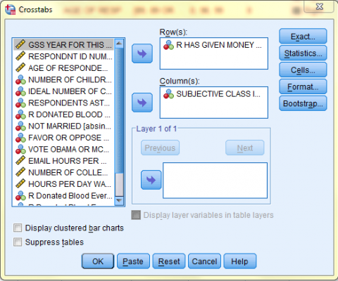
In the Crosstabs dialog box that pops up, select one of the variables of interest (R Has Given Money To A Charity, givchrty) from the list of variables and bring it over to the 'Row(s):' field, and select the othe variable of interest (Subjective Class Identification, class) from the list of variables and bring it over to the 'Column(s):' field. (The placement of the individual variables into the Row and Column fields is arbitrary.) Then, click 'Statistics...'

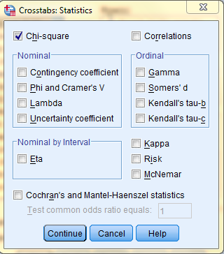
In the Crosstabs: Statistics dialog box, click 'Chi Square' and click 'Continue.'

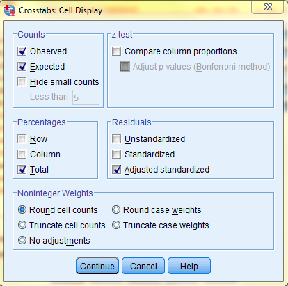
Then, back in the the Crosstabs dialog box, click 'Cells...' In the cells dialog box, in the 'Counts' field, click to select both Observed and Expected, and in the 'Percents' field, select the desired percent values you would like to be displayed in the output. Additionally, select the desired residuals output in the residuals field. Then, click 'Continue, and back in the Crosstabs dialog box, click 'OK.'

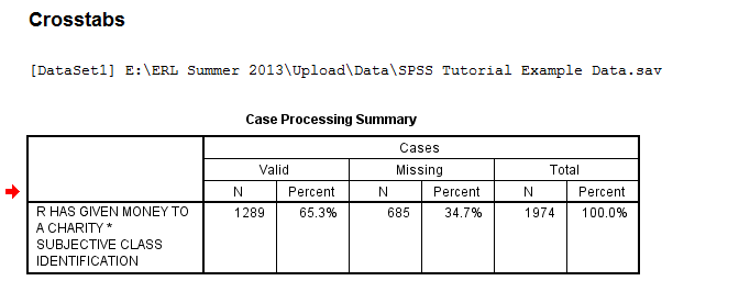
The output is displayed in the SPSS Viewer window. The output consists of three tables. The first table, Case Processing Summary, displays the number N and percent of valid cases, missing cases, and total cases in the Chi-Square analysis.

The second table, the Crosstabulation matrix, presents the counts, expected counts, and the adjusted residual (the standardized difference between the observed values and the expected values), as well as percents for each group. 

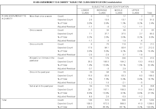
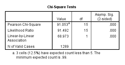
The third table, Chi-Square Tests,  presents the df (degrees of freedom), Asymp. Sig. (2-sided) for the Pearson Chi-Square value as well as other statistics. If the level of significance for the Pearson Chi-Square statistic is above .05, the probability that the difference between the Observed N and Expected N value was due to chance is 5% or less. In this case, the  Sig. value is below .05. However, the output does not explicitly indicate how the relationship exhibited in the sample data differs from a random expected pattern. The adjusted residuals in the above chart are important in determining how the relationship exhibited in the sample data differs from that of a random pattern: When the adjusted residual is greater than or equal to 1.96 (or less than or equal to -1.96), then the observed frequency value is significantly different from the expected frequency. Furthermore, if the adjusted residual value is positive, then the group is over-represented, and if the value is negative, then the group is under-represented. For example, the lower class giving money to charity once a month, a group which has an adjusted residual of -2.6, is significantly under-represented.