Data Manipulation Basics

Worksheets vs. Workbooks

An Excel file is called a workbook and will hold as many worksheets as available memory will allow (new file default is 3 worksheets). Worksheets can be independent of each other, in that the data in each worksheet is separate from the other worksheets, or they can be linked, which means that the data in one worksheet is used in some way in the other worksheets.

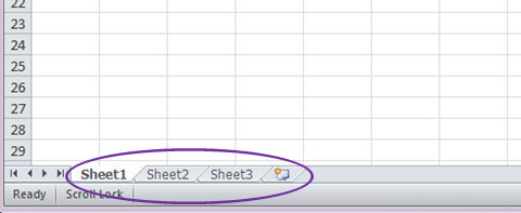
Having multiple worksheets within a workbook allows you to store different data sets together. For example, you might store each year's budget in one workbook with a worksheet for each year (these would be independent). You'll have all the data in one file if you want to review changes over the years.

Or you may be interested in analyzing information from different data sets. For example say you are interested in how unemployment rates affect wages, you may have worksheets set up like this, where analysis allows you to combine the relevant parts of each data set for analysis (these would be linked worksheets):

Or you may be collecting data from individuals and each worksheet could represent a participant in the study (each identified by a subject ID number):

You might also use one worksheet for data and another worksheet for graphs, especially if you will be using statistical software such as SPSS or STATA to analyze the data. Having graphs in the worksheet with the data can affect the importability of the data into statistical software programs, but you can eliminate those problems by importing the data worksheet and creating graphs in a seperate worksheet.

Saving a Workbook

There is more than one way to save a workbook.

• Click the save icon on the quick access toolbar.

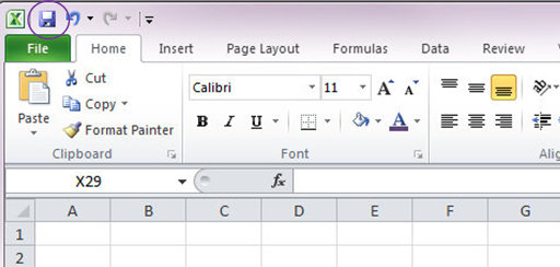
• Press 'CTRL+S' on the keyboard.
• Go to the green File tab and click on Save.

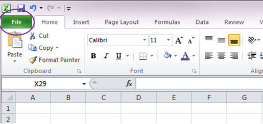
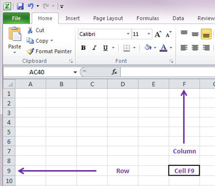
A worksheet consists of a 2 dimensional grid with columns and rows which intersect to create cells.

Columns are marked with letters. Once the first 26 columns have been labeled (A-Z), letters are doubled and then tripled to allow for 16,384 columns (up to XFD).

Rows are marked with numbers and there are over a million rows (1,048,576 to be exact). If you are attempting to work with a single data set that pushes these limits, my sympathies!

A cell is referenced by its column letter and row number.

Naming a Worksheet

There is more than one way to name/rename a worksheet.

• Double click on the worksheet tab and type in the new name.

• Right click on the worksheet tab and click on Rename.
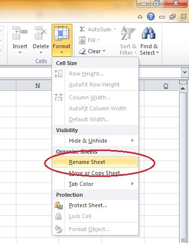
• Go to Format in the Cells group under the Home tab and click on Rename Sheet.

Adding a New Worksheet

There are many ways to add a new worksheet.

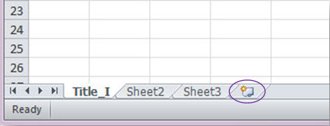
• The tab to the right of all of the other tabs has a 'new worksheet icon' on it. Simply clicking on this tab will create a new worksheet.

• Right click on the worksheet tab and select Insert…, Worksheet, and Okay to create a new worksheet to the left of the worksheet that you right clicked on.  
• Go to Insert in the Cells group under the Home tab and click on Insert Sheet. 

Deleting a Worksheet

Since there are multiple ways to delete a worksheet, choose which will be the best for you.

• Right click on the worksheet tab and select Delete.
• Go to Delete in the Cells group under Home and select Delete Sheet.

If you’ve typed anything in the worksheet, this error message will come up.

Once the sheet is deleted it is gone forever (undo is NOT an option), so always be certain before deleting that it is what you want to do.

Move a Worksheet within a Workbook

There are multiple ways to move a worksheet within a workbook:

• Click on the worksheet tab and, holding the mouse button down, drag it to where you would like the worksheet to be. A small black arrow will appear showing you where you will be placing the sheet. All information in the worksheet remains preserved during this process. 

• Right click on the worksheet tab, select Move or Copy. Then select the worksheet directly behind where you want to more the moving worksheet.
• Go to Format in the Cells group under the Home tab. This will open the same dialogue box as in option 2.

Creating a Copy of a Worksheet within a Workbook

There are multiple ways to create a copy of a worksheet within a workbook:

• Right click on the worksheet tab, select Move or Copy and select the worksheet directly behind where you want to place the copy. Check the Create a Copy box. The copy will have the same name as the original followed by a number in parenthesis, which you can rename as discussed above.

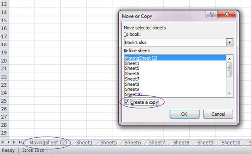
• Go to Format in the Cells group under the Home tab. This will open the same dialogue box and will refer to the worksheet you are currently in.

Move or Copy a Worksheet to a Different Workbook

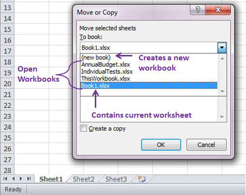
After opening the dialogue box for moving a worksheet within the same workbook (using one of the methods discussed above), open the dropdown menu to select the workbook you would like to move the worksheet to. The workbook must be open to appear in the menu. You can also create a new workbook in the dialogue box. 

To leave a copy in the current worksheet check the Create a copy check box, otherwise the worksheet will be removed from the current workbook and moved to the chosen one . 

Changing the Worksheet Tab Color

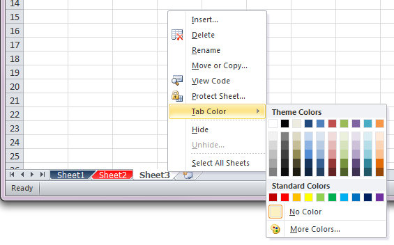
Right click on the sheet tab and go to Tab Color and select the color you would like. Note that the colors are very pale when you are working in the worksheet, but brighter in the worksheets you are not currently in. 

The Ribbon is the panel at the top of the document. There are nine tabs, and each contain a different set of features that will help you in editing and developing your spreadsheet. 

The features in each tab are categorized into related groupings (hereafter referred to as a group), such as Font, Alignment, and Number all found in the Home tab. Some features are displayed in the Ribbon, while others can be reached by clicking the small arrow in the bottom right corner of the box of some of the groups. No arrow means there are no more functions associated with that grouping. 

Note: CTRL+F1 minimizes or restores the Ribbon.

The Ribbon can be customized if there are certain features you would prefer to have in the Ribbon over others. This will be discussed later in the tutorial.

Entering Data

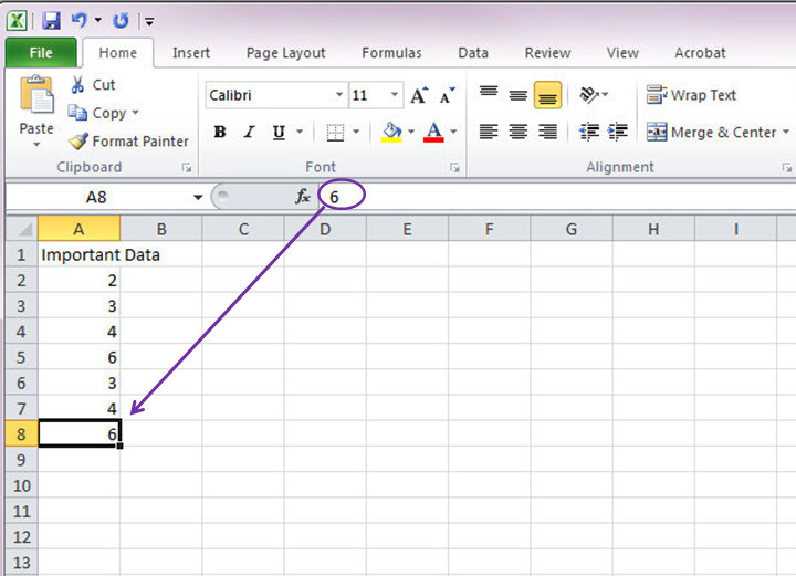
To enter data into a cell, simply type it in. When you type into the cell, the information will also be visible in the formula bar.

Use the arrow keys to move from cell to cell. Also, pressing ENTER will move to the cell below and SHIFT+ENTER will move to the cell above. Pressing TAB will move to the right cell and SHIFT+TAB will move to the left cell.    

If your mouse has a scroll wheel (the "third" button) you can use it to scroll up and down the spreadsheet (but not change which cell you are typing in). When you hit the SCROLL LOCK key (if your keyboard has one) you can use the arrows to scroll up, down, left, or right (but not change which cell you were typing in).   

Selecting Cells

There are many ways to select cells in a worksheet.

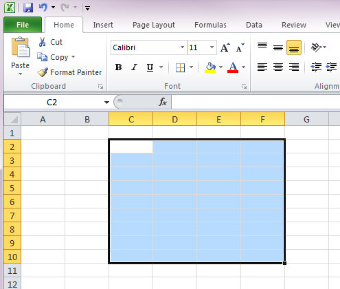
• Use the mouse to select a range of data cells. Click on the cell in one corner of the range and holding down the mouse key, drag the mouse until all cells in the range are highlighted.
• Select the cell in one corner of the range and while holding down SHIFT, either use the mouse to click on the cell in the opposite corner to mark the range, OR use the arrow keys to highlight the cells. 

Selecting Non-adjacent Cells

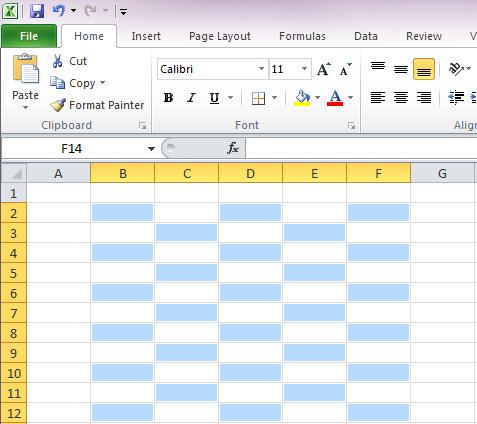
To select cells that are not next to each other, click on the first desired cell (or range of cells), and then while holding down CTRL, click on the other cell (or range of cells) As long as you hold the CTRL key down you can continue selecting non-adjacent cells. However, not all functions can be performed on multiple cells (e.g. Paste). 

Selecting Rows or Columns

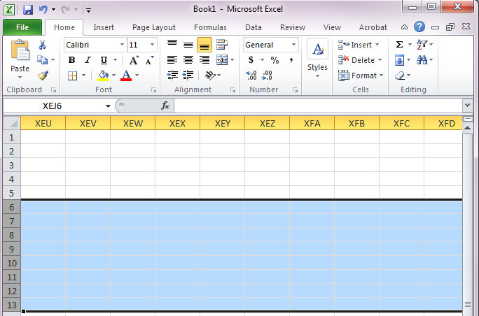
To select an entire row, click on the number of the row with the mouse. This will select all cells in the entire row (all the way to XFD). Holding down the mouse key you can also highlight multiple rows by scrolling down the numbers.

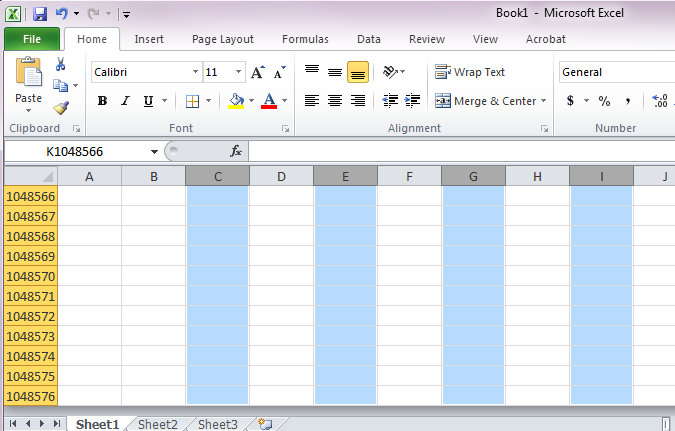
Selecting columns works in the exact same way except that you replace numbers with letters.

As with cells, you can highlight non-adjacent rows by pressing CTRL and clicking on the numbers of the rows you want to highlight.

Selecting the Entire Worksheet

Press CTRL+A and all of the cells in the worksheet will be highlighted. You can also click on the top left corner of the worksheet (directly above the 1 and directly to the left of the A). 

Changing the size of cells

Select the rows, columns or range of cells that you want to change the size of (note that changing the size of a range of cells will automatically change the size of the entire row(s) and/or column(s), not just the selected range). Go to Format in the Cells category under the Home tab.

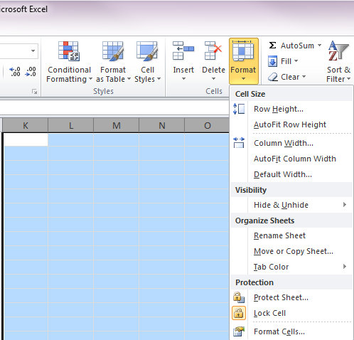
When you click on Row Height (or Column Width) a dialogue box opens with the current row height (or width) where you can type in the new height (or width).

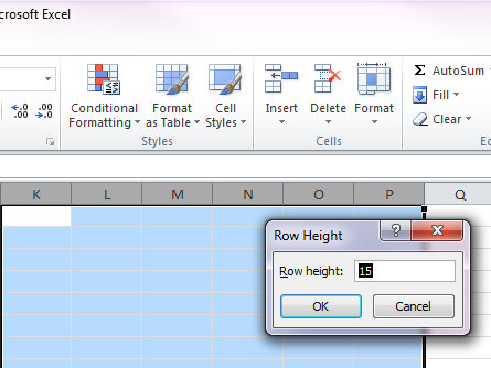
All of the selected rows (or columns) will change. 

You can also change the row height (or column width) with the mouse, but you must select either columns OR rows, NOT a range of cells. After selecting the columns (or rows) you can scroll the mouse over the column letters (row numbers) and the cursor will change to look approximately like this when it scrolls over the borders between columns (or rows): 

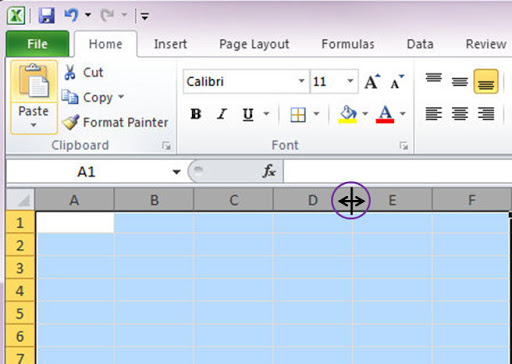
Holding down the mouse you can drag the column (or row) to be the width that you want. You can also double click on the double arrow cursor and the columns will automatically fit to the size of the contents in the cells. All selected columns (or rows) will be changed.

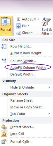
AutoFit Column Width is also an option under Format in the Cell category under the Home Tab and will do the same thing. 

Making Numbers Visible

Sometimes in Excel you'll get this:

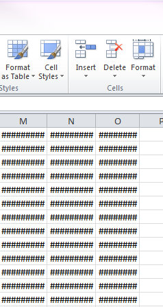
This happens when the size of the number is wider than the width of the cell. You can format it by using the methods described above and then

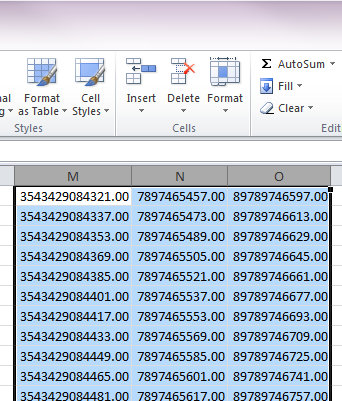
You will be able to see all of your numbers!

Font

In the Font group in the Ribbon you can easily change the font type, the font size, the font color, the cell color (background color), and the font "texture" (bold, italics, underline). 

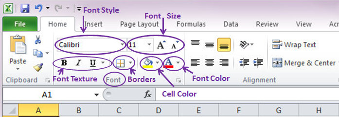
There are a few more font formatting options that you can access by clicking the small arrow in the right bottom corner of the Font group. The Format Cells dialogue box that opens has a number of tabs. In the Font tab, there are additional font formatting options such as changing the underline type or striking through information in the cells. Text can also be changed to superscript or subscript. The Border tab and Fill tab also give you more formatting options than the Border and Fill links in the Font group in the Ribbon. 

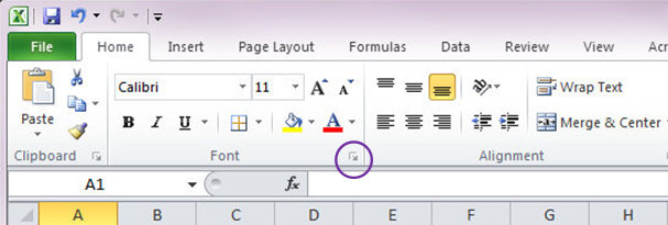
Additionally, when you right click on a specific cell or a group of selected cells and go to Format Cells..., the same dialogue box opens.

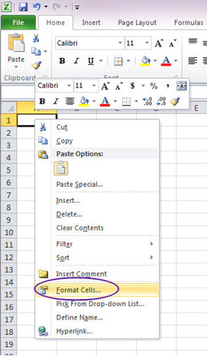
Alignment

Alignment is both a group in the Ribbon and a tab in the Format Cells dialogue box.

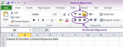
Alignment allows you to align text (and numbers) in cells to the left, center, or to the right of the cell (horizontal alignment). It also allows you to align text towards the bottom, top, or center of the cell (vertical alignment). The different allignment options can be very useful for formatting data for readability. Also in Alignment is Wrap Text. Say you have a column header that is very long. You could increase the width of the column to see it in its entirety (see above) OR you could wrap the text so that it fit in the width of the column by making the row larger. 

Here we have 3 headers, but only the final one can be read completely. 

If we highlight the cells and select Wrap Text...

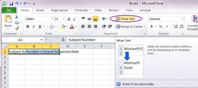
You get:

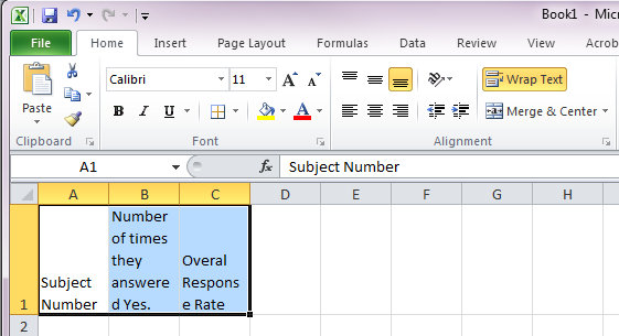
You can alter the column width so that words are not cut off. You can also set the horizontal and vertical alignments to your preference. In the Alignment group you can also change the orientation of the writing by clicking text orientation button. The dropdown arrow will give you orientation options. You can also change the indentation of the text by clicking on the indentation buttons just below the orientation button. Also, notice that the text was vertically centered in the following example. Selected Alignment items are highlighted in yellow.

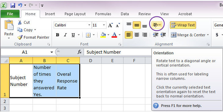
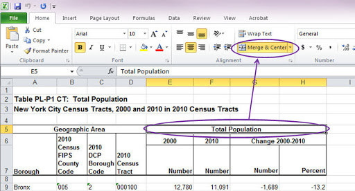
Finally Merge & Center will allow you to merge selected cells and center the context in the newly created larger cell.

Number

Number is both a group in the Ribbon and a tab in the Format Cells dialogue box.

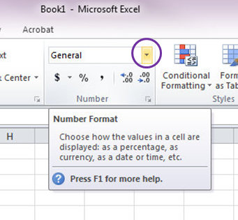
Number allows you to format cells to different data types (general, date, time, number). By clicking on the arrow next to the Number Format bar (with default option "General") you can find many number formatting options, as well as More Number Formats, which will take you to the Format Cells dialogue box.

In Number you can also adjust the number of decimal points, add monetary signs, change to a percent (which multiplies the information in a cell by 100 and adds %), or add commas (changing 1000 to 1,000).

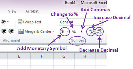
You can change the monetary symbol by clicking the arrow next to it to open a menu for a few options and the option to open the Format Cells dialogue box for even more options.

Copying & Cutting

Select the data (cell, cell range, row(s), or column(s)) that you would like to copy or cut (for help selecting, click here). You can copy nonadjacent cells, but you cannot cut them. You will get this error message when you try to cut nonadjacent cells.

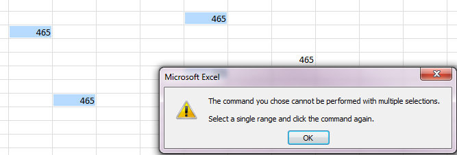
This will also happen sometimes if you are selecting multiple non-adjacent rows or columns and unintentionally click on a cell instead of the row number or column letter. You will have to restart the selecting process if this happens.

When you copy information it will remain in the original location after it is pasted, whereas if you cut the information it will be removed from the original location after you paste it. Cut will not remove the information if you do not paste (to delete information scroll down). 

Once you've selected the relevant data, there are 3 ways that you could Copy or Cut:

1.  Right click the mouse to open this menu and select Copy or Cut.

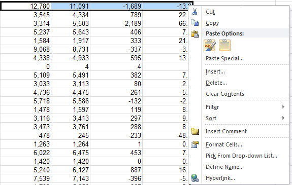
2.  Press CTRL+C to Copy and CTRL+X to Cut.

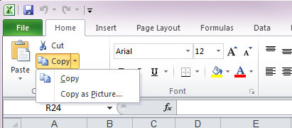
3.  Select Copy or Cut from the Clipboard group in the Ribbon. Copy has a dropdown menu that also allows you to Copy as Picture...

When you Cut or Copy information it is stored in the Clipboard. This is different from the Clipboard group in the Ribbon. You can open the Clipboard by clicking the small arrow in the bottom right corner of the Clipboardgroup under the Home tab. This will show you everything that you cut and copied.

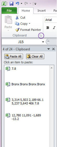
This is convenient if you will be pasting different pieces of information over and over again. By having the Clipboard displayed you can simply put the cursor in the cell in the worksheet where you want to paste the information and then click on the item in the Clipboard. It will paste there automatically. You can continue to see the Clipboard when you switch between workbooks so that if you were copying, cutting, and pasting information in one workbook and want to also paste some of the information in another, you could do so. Please note that when pasting by clicking on the item on the Clipboard it will not paste a formula, but simply the outcome of the formula (more about formulas later). 

However, you can Cut, Copy, and Paste without ever looking at the Clipboard.

Paste

Now that we've covered the ins and outs of cutting and copying... we must paste! As with Cut and Copy there is more than one way to Paste.

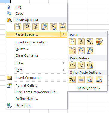
1. Right click on the cell(s) into which you would like to paste, and the dropdown menu will appear. You will see the Paste options are far more extensive than Cut and Copy (each yellow clipboard is a different paste option). By scrolling the mouse over Paste Special you get even more options.

If you scroll over one of the yellow clipboard icons of Paste Options, Excel will show what the pasted data will look like. For example, these copied rows

will transpose to look like this when I scroll over the Transpose option:

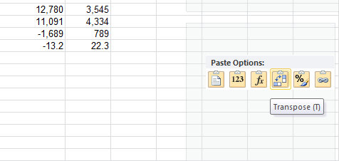
You can't see the rest of the menu, but you can see how the to-be-pasted cells will look.

Another important feature is to be able to paste just the values into your excel sheet. You might want to do this if you have formulas calculating the entries to some cells (like averaging over nearby cells) and you want to use these values for another calculation, in another sheet, or even export for use in another program. For this, you will Paste as Values from the menus above (or the alternate menus below). 

Additionally, you can click on Paste Special to open this menu:

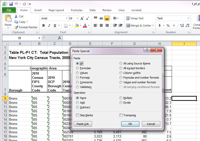
Many of these options were presented by the yellow clipboards.

2. You can also Paste by typing CTRL+V. This pasting option will conform to the data type that you are pasting. For example, a number will remain a number, a formula will remain a formula, and a date will remain a date. 

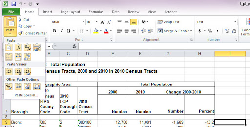
3. Click on the Paste icon in the Ribbon in the Clipboard group.  There is an arrow under the icon that will open the options also found in the menu when you right click on the cell.

Inserting Rows or Columns

Inserting rows and columns is slightly different than inserting a cell or cell range. So we'll start with rows and columns. The instructions and examples that follow are for columns, however it is basically the same for rows. Replace column with row and right with under.

There are multiple ways to carry out the following function.

• Select the column to the right of where you want to insert a new column. (Go here to remind yourself how to select the entire column.)

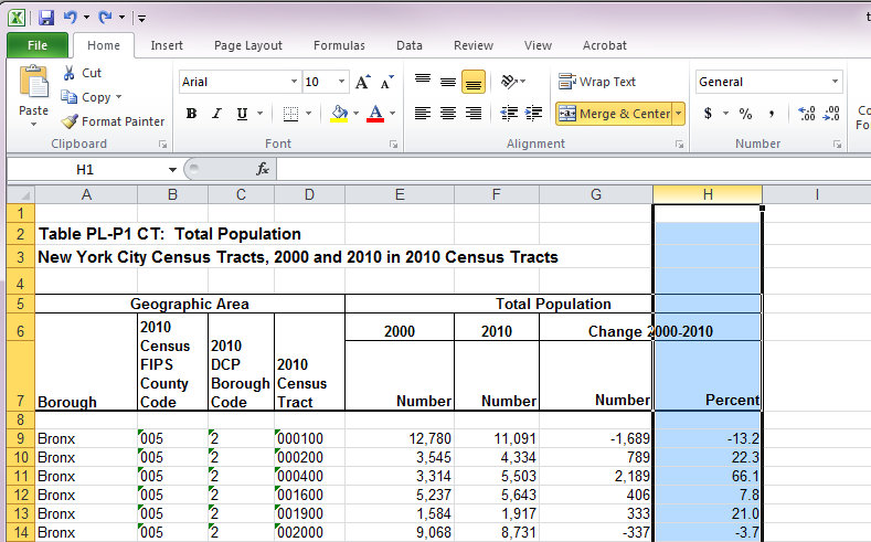
Right click on the mouse and select Insert.

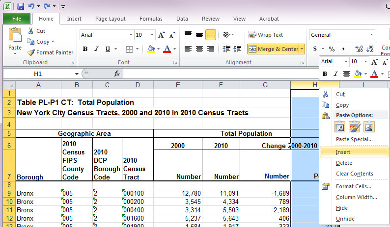
The new column will be inserted.

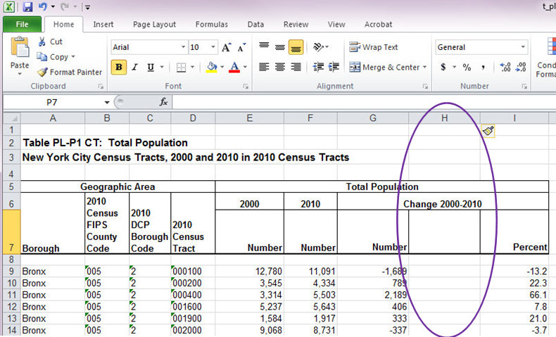
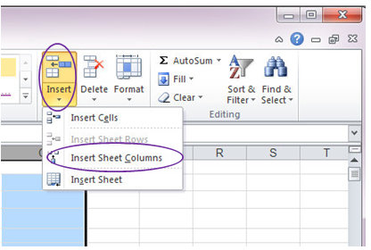
• Select the column to the right of where you want to insert a new column. Then click on Insert in the Cells group in the Ribbon. It will automatically add a column because you have selected a column. Insert also has a dropdown menu in which you can select to insert cells or a worksheet in addition to a column.

You can also insert more than one column at a time. For example, if you want to insert 3 adjacent columns here.

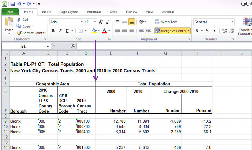
Highlight three columns starting with the column immediately to the right of where you want the inserted columns to be.

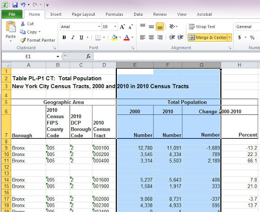
Then either right click on the mouse and select Insert or click on Insert in the Cells group in the Ribbon.

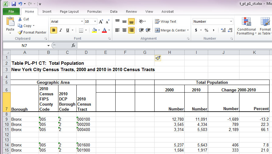
Three blank columns appear maintaining the format of the selected columns.

You can also insert non-adjacent columns (for selecting nonadjacent columns go here). It can get a little tricky predicting where the new columns will be inserted. Columns will always appear to the left of the selected columns. For example, with these columns selected

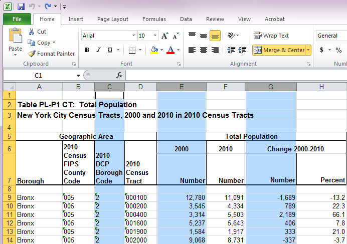
you get these columns inserted.

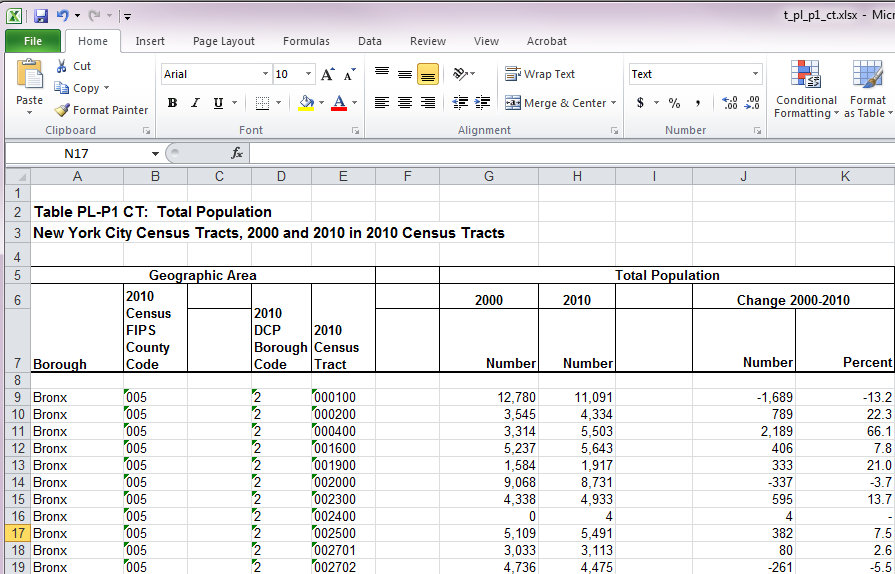
If you had anticipated having an inserted column every other column, you didn't get it. But you'll notice that there is an inserted column to the left of the '2010 DCP Borough Code' column, to the left of the 2000, Number' column, and to the left of the 'Change 2000-2010, Number' column, which were the three selected columns.

Remember that the process for inserting rows is the same; simply replace rows with columnsand right with under (or left with above).

Inserting Cells and Cell Ranges

Essentially, the process for inserting cells is the same as the process for inserting rows or columns. Say you wanted to insert a range of cells between the Brooklyn and Bronx data in the example below but you didn't want to affect the data to the right. Inserting new rows would add new rows to that data as well. Instead, you can insert a cell range.

Select the cell range the size that you would like to insert (in this case we are inserting a 4 x 8 cell range). Start the selection immediately below where you want the cells inserted because we are inserting a range of cells instead of rows.

As with inserting rows and columns you can either right click the mouse and select Insert or you can click on Insert in the Cells group in the Ribbon. If you click on Insert in the Cells group, it will automatically shift the cells down. If you right click the mouse and select Insert, you'll get this message:

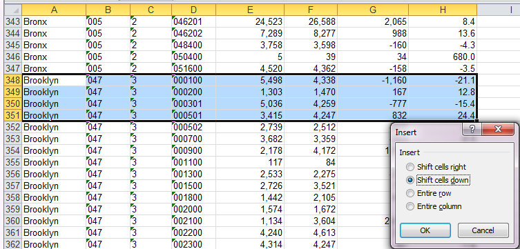
In this example, we want to shift the cells down, however, there are situations in which you will want to shift the cells to the right. By opening this menu you can specify which you want, in case the default action when you click Insert in the Cells group is not the one you want. You can also reach this menu by clicking the arrow under Insert in the Cells group and selecting Insert Cells. 

The default when you click Insert in the Cells group is not always to shift downwards. The default direction is based on your selection.

When new cells, columns, or rows are inserted, references (e.g. formulas relating to the cells) will adjust accordingly (see formulas for more on this).

Deleting Rows and Columns

Deleting works in very much the same was as inserting except that you click on Delete instead of Insert. 

Say you wanted to delete the selected rows.

There are multiple ways to do this. You could:

• Right click on the mouse and select Delete. 
• Click on Delete in the Cells group in the Ribbon. 

This will remove the rows, including their content, causing everything below to shift up 2 rows. When columns are deleted all columns to the right are moved leftwards.

Deleting Cells and Cells Ranges

Say you decided you didn't need to have those extra cells between the Bronx and Brooklyn data after all, but you couldn't delete the whole rows because you still have that data set to the right. You select the cells you want to delete.

There are multiple ways to do this.

• Right click on the mouse and select Delete. This will give you a similar menu as when you inserted except it will say Delete and it will specify opposite directions for moving cells (move them up instead of down or left instead of right).

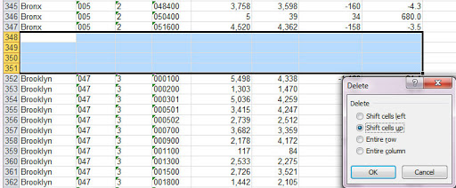
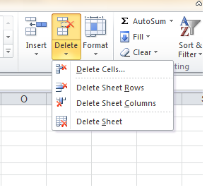
• You can also click on Delete in the Cells group in the Ribbon with the same caveats as mentioned when inserting (the default direction may not be the direction you wanted), or clicking on the dropdown menu under Delete and selecting Delete Cells to open the same menu in the image above.

Delete Content Without Deleting Entire Row

There are multiple ways to do this.

• Press DELETE or BACKSPACE.
• Right click the mouse and select Clear Contents. This will remove content but not the actual rows.
• Select Clear in the Editing group under the Home tab in the Ribbon. This will automatically provide a dropdown menu.

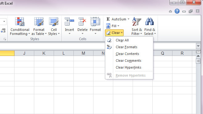
• You can also delete the contents of a cell while still entering the information (before pressing ENTER) by pressing ESC.

Undo, Redo, & Repeat

Undo

Sometimes we do things we wish we didn't. But in Excel we can undo them (usually)! As with most things in Excel, there is more than one way to do it.

• Click on the icon on the Quick Access Toolbar. You can also click the arrow next to the icon and select to Undomany items at once. (If this is not what your Quick Access Toolbar looks like, instructions for changing it are here.)

• Press CTRL+Z to Undo the most recent action.

Some actions cannot be undone (e.g. Save). When there is nothing to undo or it can't be undone, the undo button in the Quick Access Toolbar becomes gray or you'll hear a ding or beep when pressing CTRL+Z.

Redo

Redo pertains to actions you undid, but wish you hadn't, not to actions that you did and would like to do again (this is Repeat and logically the two are very much related).

• Click on the icon on the Quick Access Toolbar (which it is blue, because otherwise, there isn't anything that you can Redo). As with Undo you can click on the dropdown arrow and Redo many items at once. (Follow this to change the Quick Access Toolbar)
• Press CTRL+Y to Redo the most recent Undo (note that CTRL+Y also Repeats, see next section).

Repeat

Repeat allows you to repeat an action you just did. Repeat only repeats that most recent action once. If you want to repeat the same action multiple times, you might be better off creating a Macro.

The Repeat icon is not on the Quick Access Toolbar by default, but you can click the link or scroll down to the Customize Quick Access Toolbar section to learn how to add it.

• Once inserted in the Quick Access Toolbar, click the Repeat icon where you want to repeat your last action.
• Press CTRL+Y to Repeat the most recent action once. This action works for both Repeat and Redo because of the relationship with Undo. If you undo something, you can't repeat that action, but you can redo it. If you haven't undone anything, then there would be nothing to redo, but you could repeat the previous action.

Be aware that not all actions can be repeated.

Customize Quick Access Toolbar

The quickest way to customize the Quick Access Toolbar is to click on the dropdown arrow to the right of all of the icons on the toolbar.

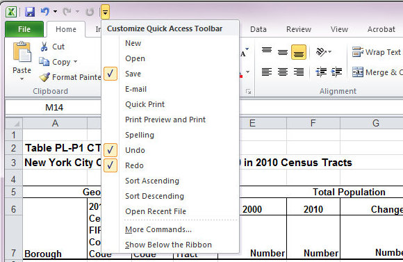
Click on More Commands. 

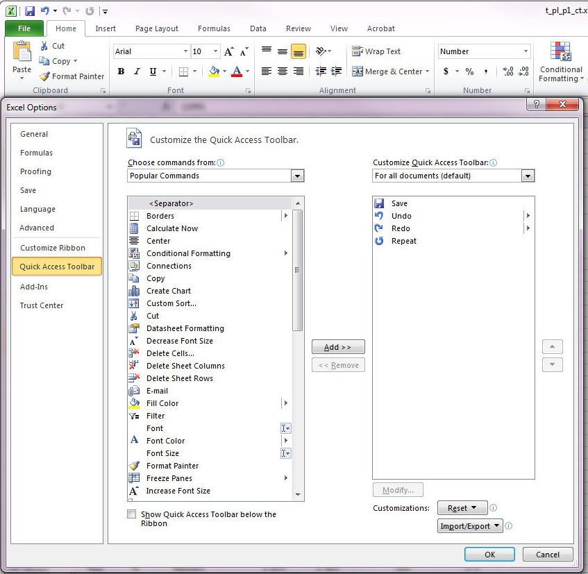
The column of items to the left contains everything that you could put in the Quick Access Toolbar. Select the item you would like and click the Add>> button. You can only add one item at a time. You can also remove items from the Quick Access Toolbar by selecting the item you would like to remove from the column in the right and clicking <<Remove. 

You can also edit the Quick Access Toolbar by clicking Options under the File Tab. In the new dialogue box click Quick Access Toolbar in the left column.

Find & Replace

Find

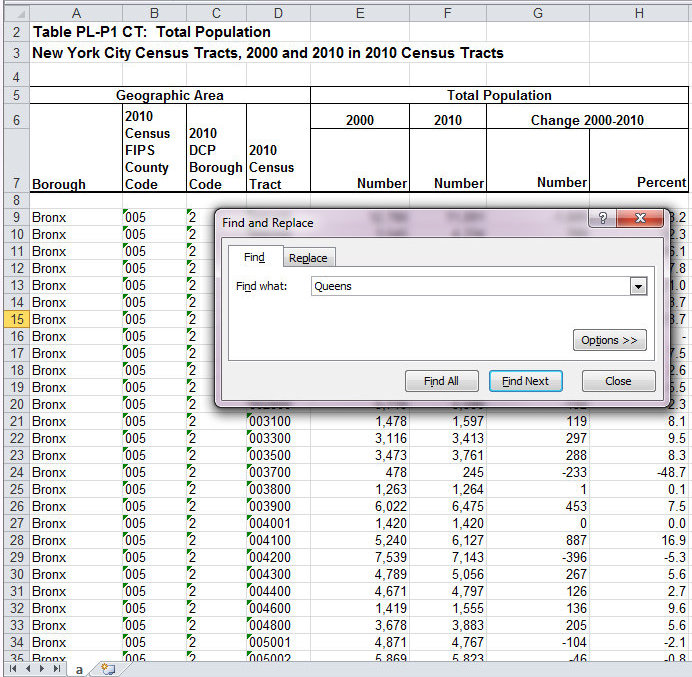
Sometimes it is useful to know how to find something quickly in a file. For example, let's say you are looking at the data file of the Census information from the 5 boroughs of New York for 2000 and 2010 displayed below and you wanted to look at data about Queens. You could scroll down the worksheet until you see it, or you could dearch for 'Queens' using Find.

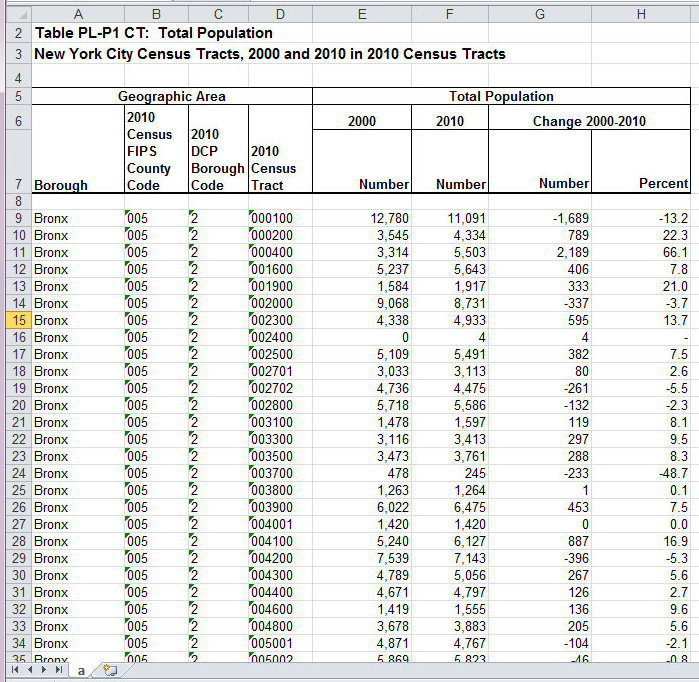
Press CTRL+F on the keyboard. This opens a dialogue box where you can type in the term or number that you are searching for. In this case, we would type in 'Queens'.

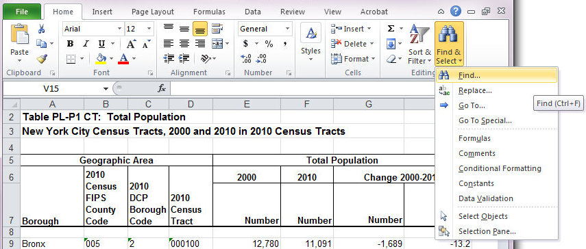
This dialogue box can also be reached by clicking on Find & Select in the Editing group on Ribbon and selecting Find from the dropdown menu.

In the Find and Replace dialogue box you can click on the Options>> button to modify the search results.

Let’s say, for example, you are interested in finding all of the instances in which the Total Population did not change between 2000 and 2010. To do this, you need to search for zeros in column G (which represents the change in total population between 2000 and 2010 in terms of number, instead of percent). If you simply type 0 into the Find box, you will find every single cell that contains a zero.

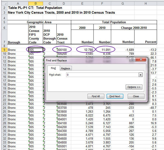
Because you want to search in a specific column (G), you should select the entire column by clicking on the letter 'G' before opening the Find dialogue box. When you click on the Options>> button you can select the check box for Match entire cell contents to search for cells that contain '0' and nothing else.  You would also select By Column from the Search dropdown menu.  Then select Find Next or Find All. 

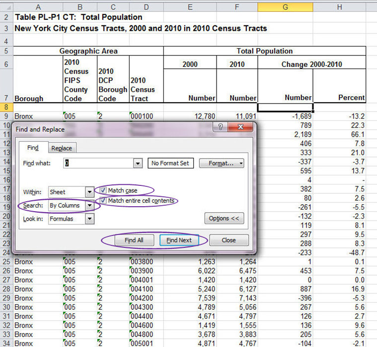
Find Next will find the next instance of 0 in column G. You could continue clicking Find Next to find and note all census tracts in which the total population did not change from 2000 to 2010.

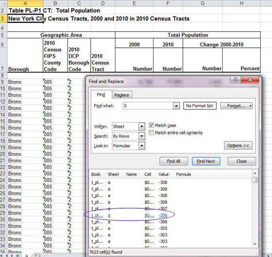
Find All will find all of the instances of the search item. When you select Find All a menu shows up below the dialogue box that shows all instances of the item you are searching for. You can scroll to the items in column G and click on the specific cell to go to that cell in the worksheet.

Replace

Replace works just like Find except that you can choose to replace an item with something else (including a blank).

Select the Replace tab in the Find and Replace dialogue box. You can also reach this by selecting Find & Selectin the Editing group in the Ribbon and then selecting Replace.

Under the Replace tab, in addition to the Find what box, there is a Replace with box in which you can enter the item (or nothing) that you want to replace the item you are searching for.

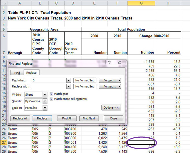
For example, let's say you are interested in calculating the average population change for each borough, but you don't want to include instances where there were no changes. In which case you could do the same search for zeros in column G as before, but Replace it with a blank. The average function in Excel will skip over blanks when calculating the average (more on that here). Select Find Next to find the first item you will be replacing.

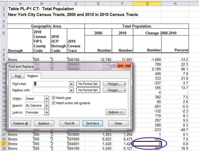
Then select Replace.

Replace All will replace all of the found items, which can be useful, but sometimes it will also replace things you weren't anticipating. In this case it would replace zeros found in cells in all of the columns, not just G, which would be problematic. If you select the entire column G, it will only replace items in that column.

Sort

Sorting can be extremely useful when working with data sets. A basic Sort will sort information in columns from smallest to biggest or biggest to smallest (or in the case of text from A to Z or Z to A). As an example, let's assume you are interested in the Census Tracts that showed the largest percent change between 2000 and 2010. Since the file is organized by Census Tract it is difficult to tell which areas showed the largest percent of growth.

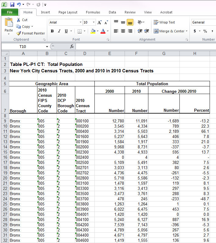
We can sort the Percent Change column (H) from biggest to smallest.

Sorting a Single Column

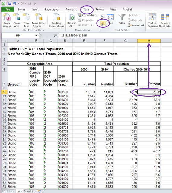
Click on a cell in the column we want to sort (H) under the headers (headers or headings are essentially the titles in the columns). Under the Data tab select the Z->A button in the Sort & Filter group in the Ribbon.

Sorted data will look like this.

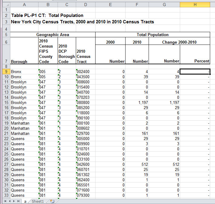
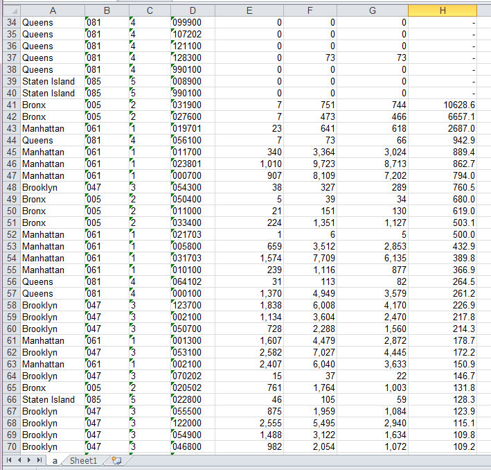
The cells with '-' were created since the 2000 census and so there is no way to measure the population change in that particular area. You could do a Find & Replace if you would prefer to change those (go to the Manipulating Data I page to find out how). When we scroll down we find the areas that demonstrated the largest amunt of growth between 2000 and 2010. You'll also notice that the boroughs are intermixed.

Data can also be sorted using the Sort dialogue box which you can get to by clicking on Sort in the Sort & Filtergroup under the Data tab.

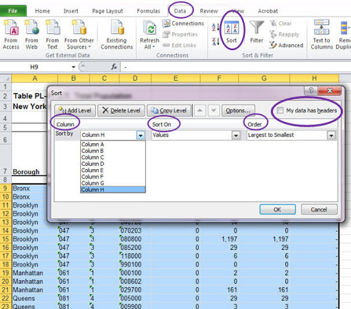
Using the dialogue box you can specify if your data does or does not have headers. You can specify the column under Column, the sorting criterion under Sort On, and the sorting order under Order. Notice that the to-be-sorted data is selected- this happens automatically IF you have selected a cell in the dataset. You can also highlight the range that you want to sort. 

Sorting Multiple Columns

You can sort multiple columns simultaneously. For example, say you wanted to look at the largest percent change as before but you wanted it sorted by borough, so that you could see the largest percent change in the Bornx, and then scroll down to Brooklyn, and so forth. In the Sort dialogue box fill in Sort by with Column A (borough names), Sort On with Values, and Order with A to Z. Then click on the Add Level button and fill in the second row: Then by with Column H, Sort On with Values, and Order with Largest to Smallest.

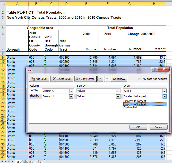
Then select OK. In the example, we've scrolled down so that you can see where the Bronx ends and Brooklyn begins. You'll notice that the since the percent change is sorted from largest to smallest, we are looking at the largest decrease at the end of the Bronx data and the largest increase at the beginning of the Brooklyn data. 

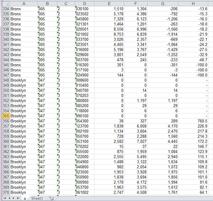
Some things to note about Sort

• Make sure all of the items being sorted are of the same data type. If you have numbers stored as text and numbers stored as numbers (see Formatting Cells for more about data types) then the numbers stored as numbers will be sorted before the numbers stored as text.
• Also be sure to remove any spaces preceeding information in the cells. Sometimes data sets will have 'leading spaces' in which there is a space preceeding the number in the cell. This can occur if the original data file was not an Excel spreadsheet.
• Be careful when sorting items that include formulas (more on that soon) because the return values could change.
• Keep column headers in one row (otherwise, you can't sort by the full column header). In our current example data, we were sorting by column names rather than headers. That is because the headers covered 3 rows. If the header is in a single row, then you will select the header title of the column instead of the column letter.
• Also note that any hidden columns (or rows) will not move until you sort, thereby changing your data set. More on hiding and unhiding below.

Auto Fill & Series Fill

One of the great features of Excel is the Fill option. Instead of re-typing the same data or formula, you can let Excel copy it into the cells (AutoFill). Or instead of typing the numbers 1-100, you can set Excel to fill them in (Series Fill).

Auto Fill

Let's say you wanted to reformat the example data so that the terms referring to the 5 boroughs were represented as numbers. Since the Bronx is first, you give it number 1. But instead of typing the number 1 for all the data points for the Bronx (and continuing with all the other boroughs), you can use Auto Fill. Type the number 1 in the first two cells.

Select the two cells. Move the cursor over the bottom right corner of the selection. It will turn into a small black plus sign. When it does, click and hold down the mouse key and drag it down to cover all of the cells that you want to have the number 1 in. You'll notice that the selection border turns gray and that there is a small box with a 1 in it below and to the right of the plus sign. This tells you what is being input into the cell.

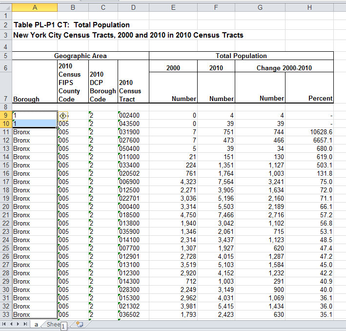
When you release the mouse key, all of the selected cells will have a 1.

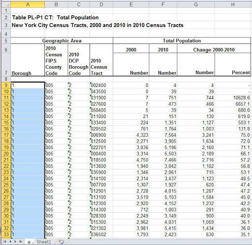
Why did you have to enter the 1 in 2 cells?  Read on to find out!

Series Fill

Say you wanted to count the number Census tracks in the Bronx and you don't completely trust your subtraction skills (remember, there is data in row 9 so you can't simply subtract 9 from the final row number of the Bronx data). But if you used a Series fill, then Excel would tell you how many Census tracks there are for the Bronx by counting each one. Type the number 1 in I9.

Click on the cell (I9) and move the cursor over the bottom right corner of the cell. When the cursor turns into a small black plus sign, click down the mouse key and drag it down until the end of the Bronx data.

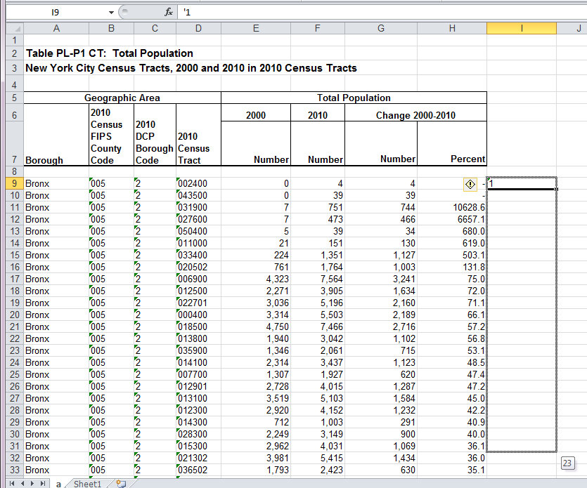
When you release the mouse key, you will see that a linear series automatically filled into the selected cells. Did you  notice the number in the small box under the cursor increase as you dragged the mouse?

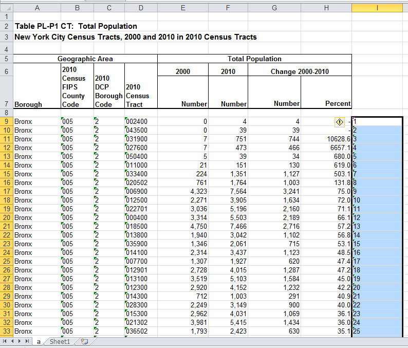
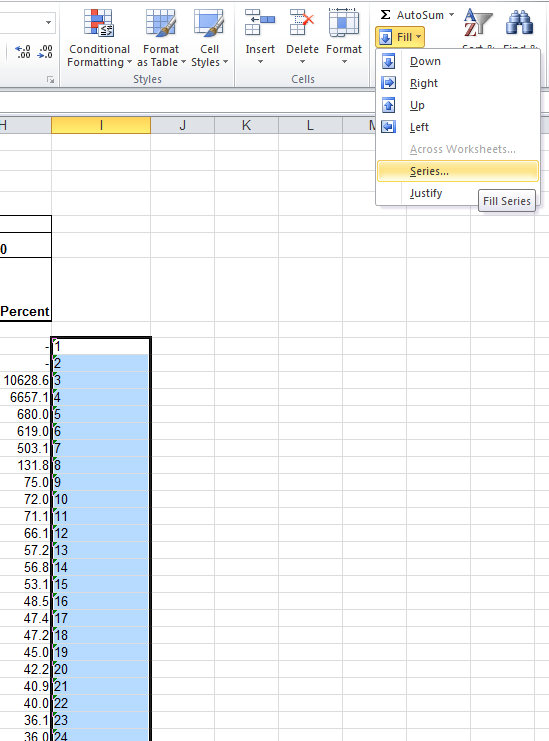
Another way that you can do a Series Fill is by going to Fill in the Editing group in the Home  tab. You’ll need to select all of the cells that you want filled in first. Then click on Fill. Select Series.

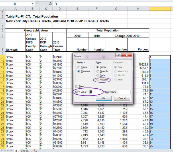
In the dialogue box that comes up you can change the parameters of the series. For example, if you wanted to increase it by 2 numbers instead of one, you would change the Step Value from 1 to 2. You can also set the Stop value or alter the Type (note that you can get to AutoFill here by selecting it under Type).

Hiding & Unhiding

There are times when you want to keep information in the worksheet, but you do not necessarily want to be looking at it. In which case, you can hide it. And anything hidden will at some point need to be unhidden (otherwise, you could just delete it).

Hiding Rows or Columns (or worksheets)

Select the row or column that you would like to hide. Right click the mouse and scroll down and select Hide. 

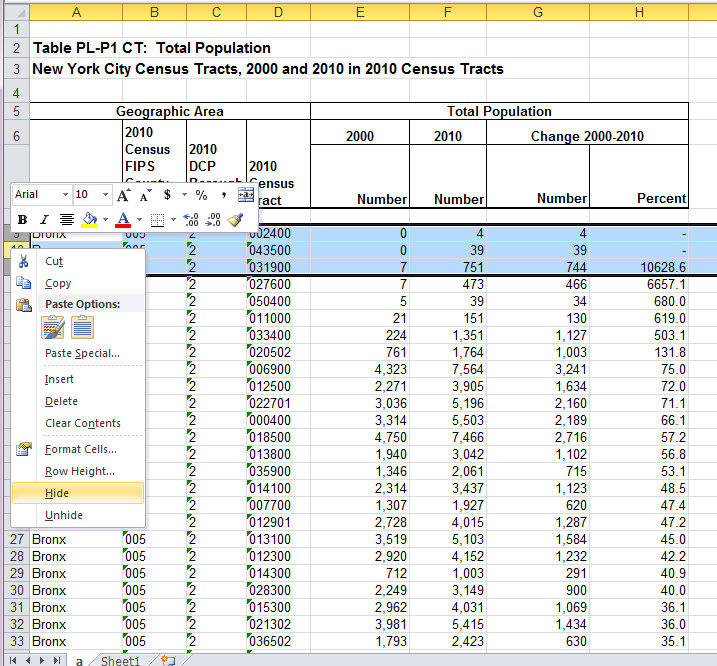
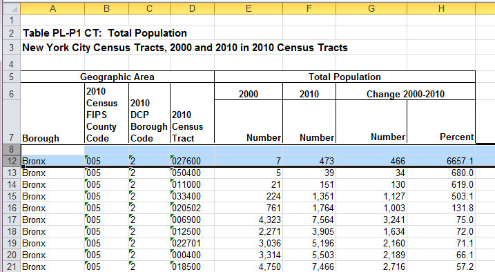
The selected row(s) or column(s) will disappear. Notice that not only does the information in the column or row disappear, but the row column letter/ row number disappears too. In this case, rows 9, 10, and 11 are hidden. This is how you can tell if there are hidden rows or columns in the dataset.

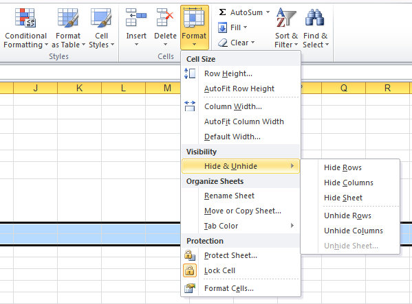
You can also hide rows or columns from the Format button in the Cells group on the Home tab. Select Hide & Unhide and then select if you want to hide rows, columns, or even the entire worksheet!

Unhide

You may want to revisit hidden information again. Also, sort will not include hidden rows or columns, so if you want to preserve the information you should unhide rows or columns before sorting.

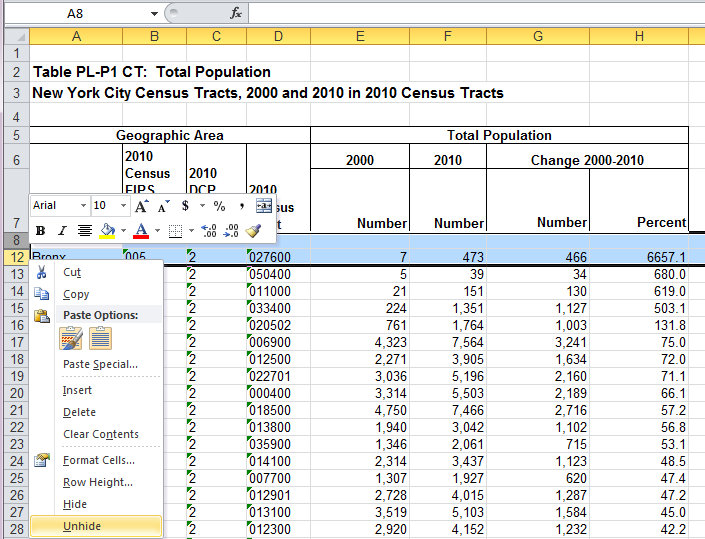
To unhide a row or column that is not the first row (row 1) or column (column A) select the surround rows or columns. So if you are interested in unhiding rows 9, 10, and 11, select rows 8 and 12. Right click the mouse and scroll down to select Unhide. 

The hidden rows or columns (in this case rows) will reappear.  As before you can also unhide columns or rows from the Format button in the Cells group on the Home tab. Select Hide & Unhide and then select if you want to unhide rows, columns, or even the entire worksheet! (Again, to unhide a worksheet, you have to CTRL+click on one of the visible worksheet tabs and select 'Unhide.')

When you select to unhide a worksheet, you will get a dialogue box listing the hidden worksheets for you to pick the one that you want to unhide. 

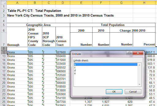
If you have hidden the first row (row 1) or column (column A) you cannot select the surround rows or columns (because what comes before row 1 or column A?). One way you can unhide them is to select all of the columns/rows. Then unhide the rows/columns from the Format button in the Cells group on the Home tab and selecting Hide & Unhide under Visibility.  Note that this will unhide every row and column. 

To unhide ONLY the first row or column, type A1 into the Name Box next to the Formula bar. From the Format button in the Cells group on the Home tab, select Hide & Unhide under Visibility, and Unhide Columns (or Unhide Rows). The missing first column (or row) will return!