Stata Tutorial

When you open Stata, the program looks like this: 

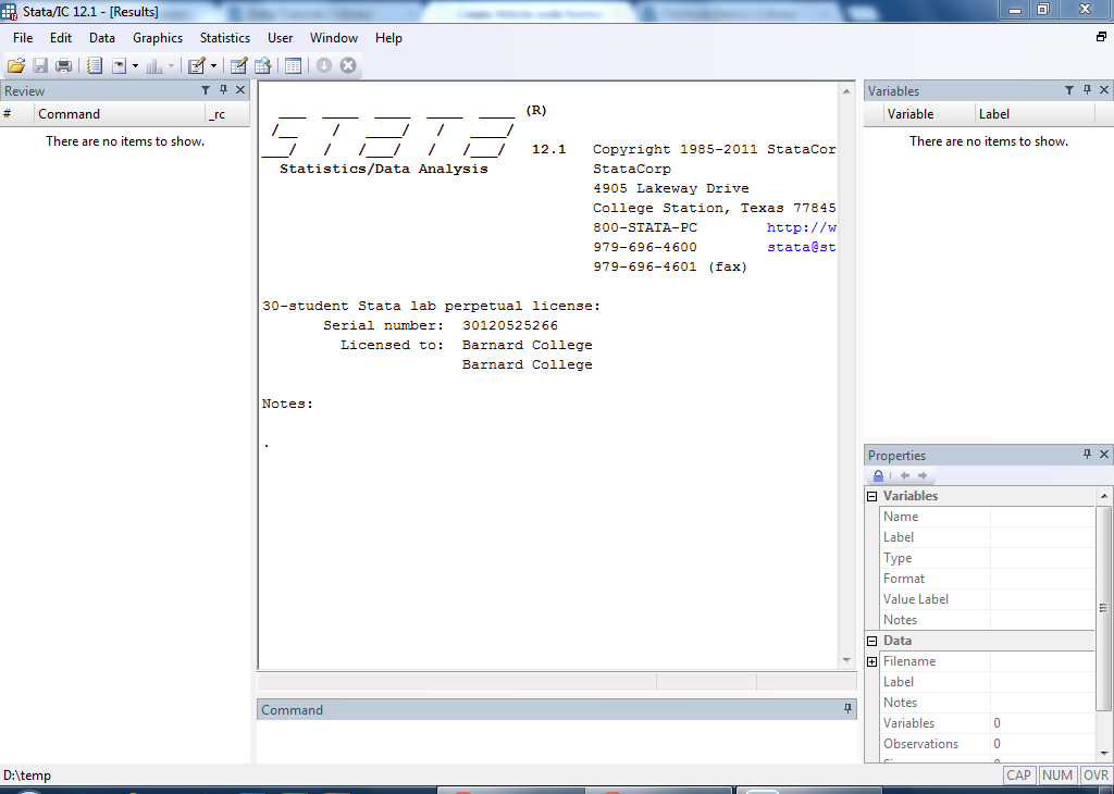
This page briefly describes what each window is for. 

Main Window

The main window is the big box in the middle of the screen. This window is the output window that displays the statistical outputs and results of all analytical procedures. 

Command Window

The small box below the main window is the Command line. This is where you can directly enter a command. We'll explain what commands are and how you use them later. For large research projects, you should use a Do File to keep track of all your commands, which will also be discussed later. 

Review Window

On the left side of the screen is the Review window. This keeps track of all the commands you have entered.

Variables Window

To the top right is the variables list. This is where you can see what variables are available in the dataset. These variables are pulled from the datase that you import into Stata. We'll explain how to import data later.

Properties Window

Finally, to the bottom left is the properties window. If you click on a variable from the variables list, the properties window will display basic information about that variable.

Creating a dataset from scratch in Stata is easy. This section describes the easiest method for beginners. 

Entering the data

Start by clicking on the "Data Editor (Edit)" button, which looks like this: 

This will bring up a window that looks like this: 

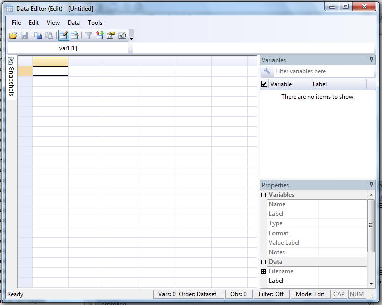
From here you can enter your data much like you would in Excel. Here's an example using data I made up: 

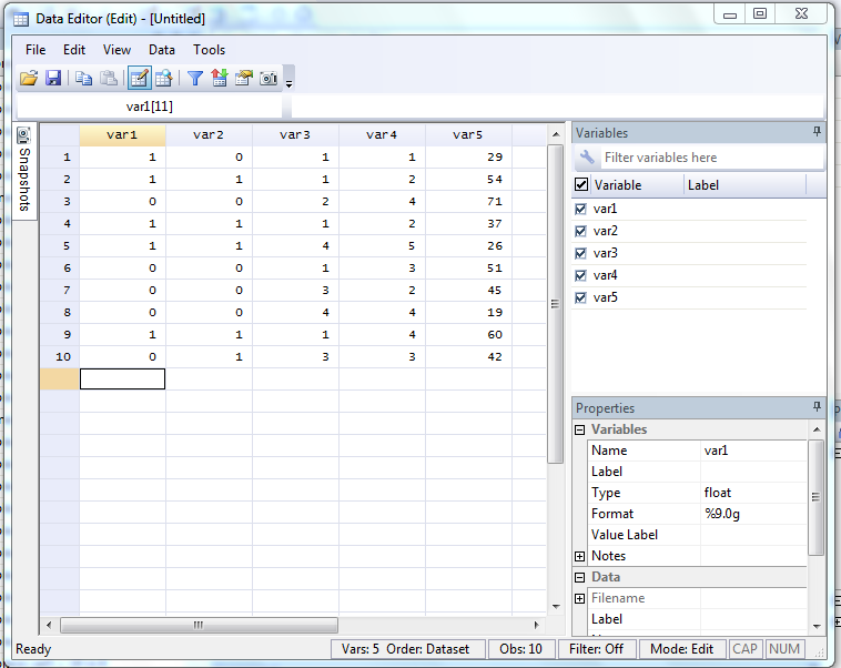
Let's assume the first column is whether someone voted for Obama or Romney, the second gender, the third race, the fourth education, and the fifth age. 

Renaming the variables

To rename the variables (which are automatically named var1, var2, etc.), click on one of the cells in the column you want to rename. In the above example, the 11th row of the var1 column is selected. We can now go over to the "Properties" box in the lower right hand corner, highlight the name "var1" and replace it with something new. Let's call it "votechoice." You can rename the same variables using the same method. Alternately, you can also now double click on the column name in the dataset ("var2," etc.) and just start typing. Hit enter to accept the new name.

You can also rename the variables using the "rename" command. If you were to close the Data Editor window and type "rename var1 votechoice," it would rename "var1" as "votechoice." In fact, this is what Stata is actually doing if you use the first method (it just runs it for you, rather than you having to type it in yourself). 

You can also now save the dataset as a .dta file if you want to have it available for future analysis in Stata.

Exploring a Dataset

This page demonstrates how to load a dataset into Stata and explore the available variables. 

Opening a dataset in Stata

If you open a .dta file on a computer with Stata, it should automatically open it in Stata. Alternately, you can type the following command: 

use "D:\TEMP\ICPSR_25383\DS0001\25383-0001-Data.dta"

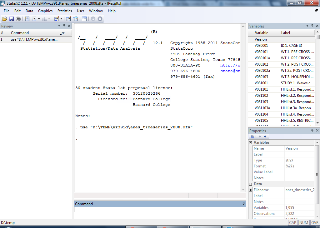
The command "use" tells Stata you want to use the dataset you type immediately afterwards. In this case, the file name of the public opinion survey I'm using is "25383-0001-Data.dta" and it is located in folder D:\Temp\ICPSR_25383\DS0001. If the file were located elsewhere, the filename in quotation marks would be different. If you're not sure where your file is located, just double click to open it and Stata will figure it out. The screen should look like this: 

Seeing what variables are there

Notice that you now have a list of variables in the Variables window at the top right. Public opinion datasets from the ANES tend to do a good job of providing usable information in this window, but it still might not be totally clear what each variable means. This is where codebooks are useful. 

Viewing the data

If you want to look at the data in spreadsheet form (think of how an Excel spreadsheet looks), you can click on the "Data Editor (Browse)" icon near the top. It looks like this: 

This brings up the Data Editor, which looks like this: 

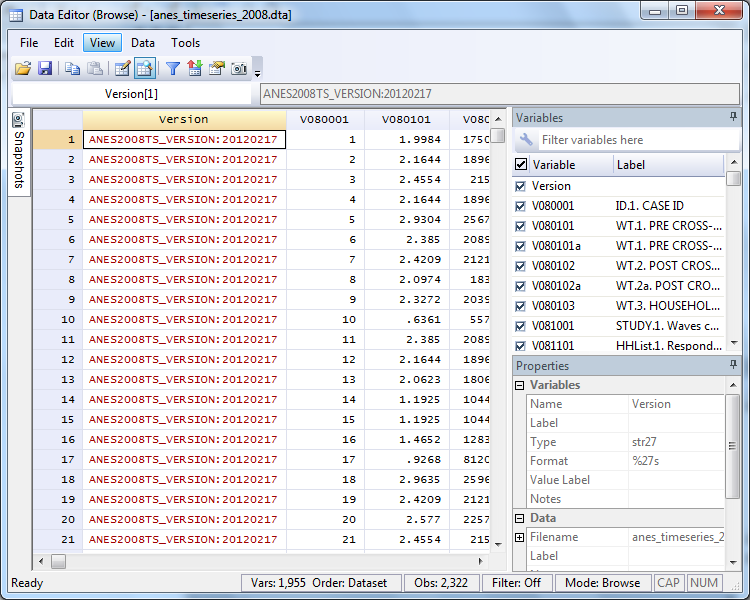
You can scroll through to look over your data. Just click the X at the top right to go back to the main Stata window. 

Frequency tables for a variable

Now that you have a dataset loaded into Stata and (in this case, at least) a wide array of variables at your fingertips, let's pick one to explore in greater detail. I'll use party identification. Variable number V083098X is the main partisan identification variable. To display a frequency table of this variable, type the following command: 

tab V083098X

The "tab" command tells Stata to create a table of the variable name you type immediately afterwards. The result looks like this: 

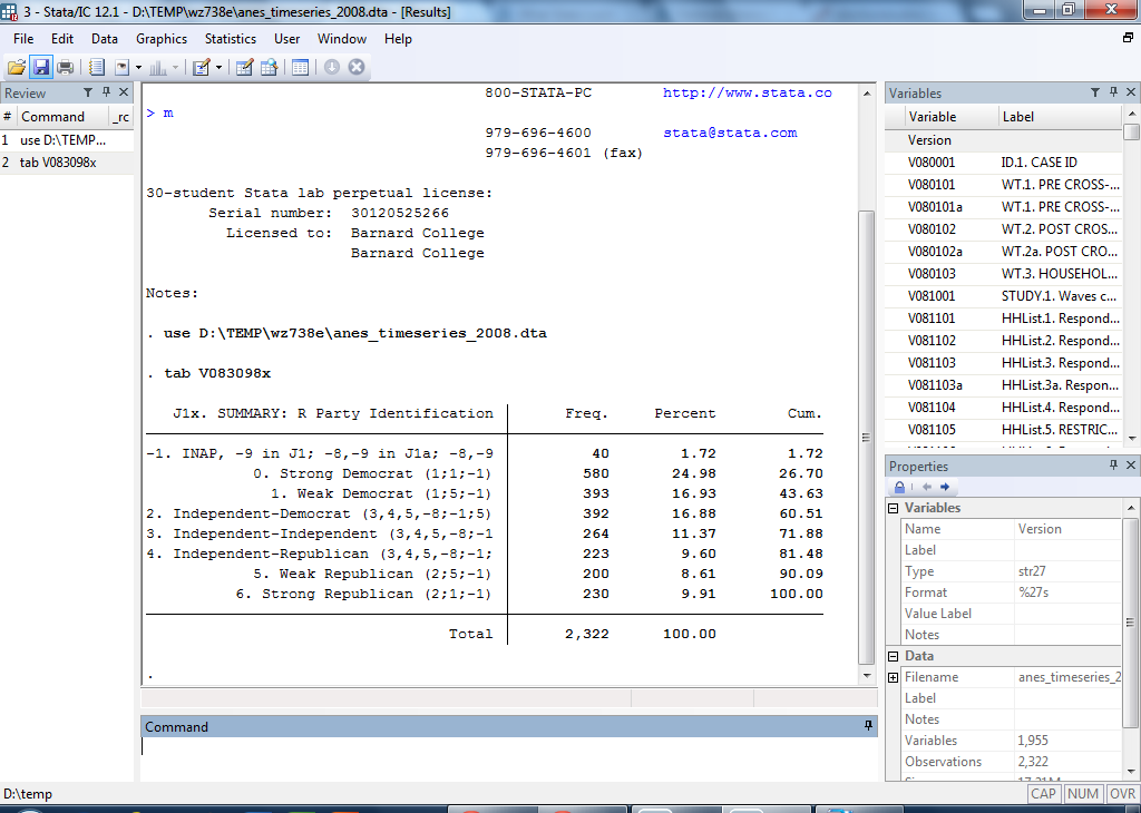
The first category ("-1. INAP, -9 in J1; -8,-9 in J1a; -8,-9") can be ignored. This category tells us that 40 people (1.72 percent of all respondents) didn't answer the question properly and thus could not be categorized. The real substance is providedby categories 0-6. In this survey, 580 individuals -- 24.98 percent of all respondents -- categorized themselves as Strong Democrat. You can also see how many identified themselves as Weak Democrat, Independent-Democrat, Independent-Independent, Independent-Republican, Weak Republican, and Strong Republican ("Independent-Democrat" means the person identifies themselves primarily as an Independent, but leans Democratic if forced to choose; likewise with "Independent-Republican"). 

Summarizing a variable

You can also obtain a number of basic summary statistics about the variable by typing the following: 

sum V083098X

Just like before, the "sum" command tells Stata to summarize the variable named immediately after the command. The result looks like this: 

This tells you there are 2,322 total observations (i.e., number of respondents) for this variable. It has a mean average of 2.239879. Its standard deviation is 2.031143. Its minimum value is -1 (that's the value ANES used to label the missing, etc., respondents) and its maximum value is 6 (that's the value ANES used to label Strong Republicans). 

Setting Up Your Research

While it is possible to simply enter each command into the Command window one by one, it's better to keep track of all your commands in one place and run them from there. Stata allows you to do this in what it calls a "Do File." Also, in many cases you need to edit and clean up the dataset before you can begin serious analysis. This page introduces you to both of these issues. 

Do Files

To open a new Do File, click on the "New Do-file Editor" icon at the top of the screen. It looks like this: 

This brings up a Do File, which looks like this: 

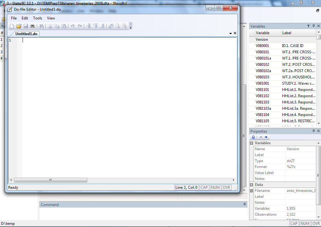
Here you can keep track of all your commands. For example, a Do File with all the commands previously run in this tutorial would look like this: 

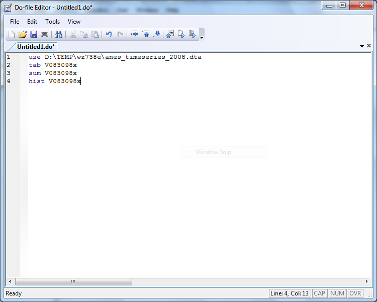
To execute a command from a Do File, highlight the command (or commands) you want to execute and click the "Execute (do") button at the top of the Do File screen, which looks like this: 

This will "do" (thus the name Do File) the files you've highlighted. 

It's best to get into the habit of working from a Do File. It might not seem obviously useful at first, but if you're working on a large research project like a seminar paper or a senior thesis it will be incredibly helpful. It allows you to immediately replicate any analysis that you have done with the click of a button. And in the event you find yourself needing assistance, sharing your Do File with one of the ERL assistants will make things much easier. 

Recoding variables

In many cases you will need to recode variables to make them useful. Consider the party identification question from the last section. It had 7 substantive categories, but the other category was actually worthless for research purposes. So even though it looks like an 8-category variable from the outset, it's really more of a 7-category variable in disguise. This biases the summary statistics (the minimum category is -1, even though that category is useless to you; it also skews the mean, standard deviation, etc.). 

So what you want to do in this case is recode the party identification variable and get rid of that category so you can focus on the actual 7-category scale. Stata allows you to do this with the "recode" command. In this case, I'm simply going to drop the -1 category and keep all the others the same. I'll name my new variable "partyid." The command to do this is the following: 

recode V083098X (-1 = .), gen(partyid)

Let's walk through the command. Like before, I begin with a command ("recode") and follow it with the variable name ("V083098X"). I next specify that I want the -1 category to be treated as missing, which in Stata means coding it as a dot ("."). I do this in parentheses. Now that I've told Stata what I want it to do to the original variable, I have to generate a new variable with a new name that has those properties. So I type a comma and a space and then use the "gen" command to generate a new variable, the name of which I place in parentheses afterwards (with no space in between). 

The output looks like this: 

Recall from the previous section that the -1 category had 40 observations, which is why there are 40 differences between the original variable (V083098X) and the new variable (partyid). Those 40 cases are now missing. 

To see this, use the "tab" command again, but this time on the new variable: 

tab partyid

The output looks like this: 

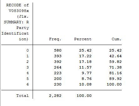
The new variable only has 7 categories (0, 1, 2, 3, 4, 5, 6), all of which are substantive (remember that they range from 0 = "Strong Democrat" to 6 = "Strong Republican"). 

Checking the summary statistics reveals a few differences there as well: 

sum partyid

Compared to the summary statistics for the original variable, the number of observations has dropped from 2,322 to 2,282. The mean is now 2.29667, compared to 2.239879 previously (having those 40 observations attached to the -1 value was weighing down the average). The standard deviation is also now slightly smaller and the minimum value is now 0 ("Strong Democrat") rather than -1 as it was previously. 

Initial Analysis

Now let's move to some real research. Let's say you're interested in the relationship between party identification -- the variable we've been using as an example so far -- and the frequency one attends religious services. To be a little more specific, let's begin with the hypothesis (which we will test here and in the proceeding sections) that people who attend religious services more frequently will identify more with the Republican Party.

So now, in addition to the party identification variable, let's introduce a new variable. The GSS asks respondents how often they attend religious services. The possible responses are never, less than once a year, once a year, several times a year, once a month, 2-3 times a month, nearly every week, every week and more than once a week. In order to see the responses, we will run a tabulation on this new variable "attend".

tab attend

You should receive the following output:

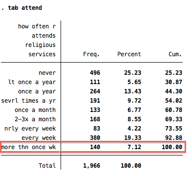
The table above shows the number of respondents that selected each response. In the highlighted box, we can see that 140 individuals out of a total of 1,966 (or 7.12% of the total number of respondents) attend religious services more than once a week.

Crosstabs

Now let's run a slightly more involved tabulation, this time with two variables. This is called a crosstabulation, or crosstab. You simply tell Stata to tab two variables rather than one. In this case: 

tab partyid2 attend

This gives the following result:

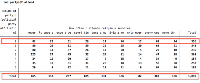
The categories for the party identification variable (partyid2) run vertically along the left side, while the categories for the attending religious services variable (attend) run horizontally along the top. If you find the intersection of category 0 on partyid2 and category never on attend, for example, you will see that 82 individuals fall into this category: Strong Democrats who never attend religious services. 356 individuals identified as "Strong Democrats" and 465 individuals answered that they never attend religious services. Therefore, of the 356 "Strong Democrats" 82 "never" attend religious services and out of the 465 individuals that "never" attend religious services, 82 identify as "Strong Democrats". You can similarly find any other combination. For instance, if you want to see how many "Strong Republicans" attend religious services once every week, simply find the crosstabulation of category 6 on partyid2 and category "every wee" on attend. Turns out there are 64 of these people in the sample. 

One clear problem with the crosstab above is they just give you raw numbers. What you should generally be more interested in is now the number of people but the percentage of respondents that make up a category. You can tell Stata to include percentages by including an additional command for row and column percentages. In this case, amend the previous command by adding ", row column" to the end, which would be this command: 

tab partyid2 attend, row column

This gives you a more detailed crosstab where you can find percentages as well as raw frequencies (this is going to take two image files because it's a big output!): 

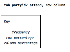
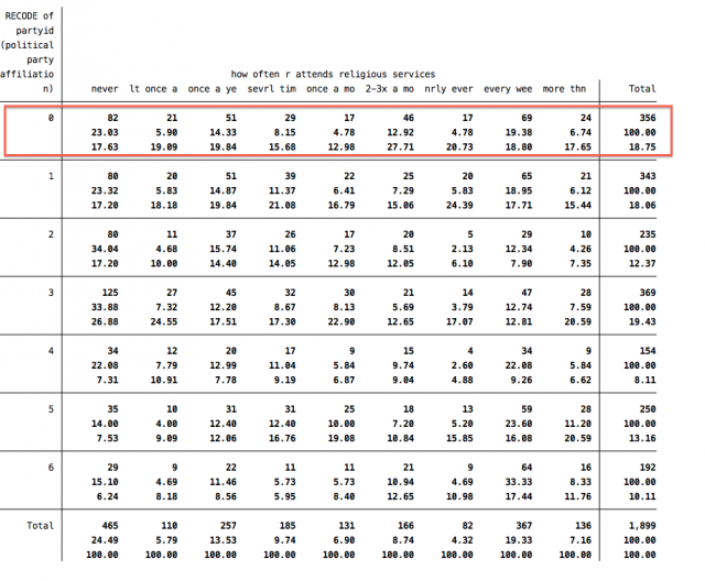
So, what do all these new numbers mean? The top number in each cell is still the raw frequency you got before you added the ", row column" bit. The second number in each cell is now the row percentage (left to right -- note how it adds across the row to 100.00 in the righthand "Total" ). The third number in each cell is the column percentage (top to bottom -- note how it adds down the column to 100.00 in the bottom "Total"). Therefore, we can conclude that 17.63% of respondents that "never" attend religious services identify as "Strong Democrats" and 23.03% of respondents that identify as "Strong Democrats" "never" attend religious services.

Also, notice that the total number of observations shown in the crosstabulation for "partyid2" and "attend" is 1,899. This number is smaller than the total number of observations for "attend" and "partyid", 1,966 and 1,906 respectively. The number of observations decreased because the crosstabulation only included respondents that correctly entered a response for "partyid2" and "attend". We can tell Stata to show us the observations that were dropped from "partyid2" in the crosstabulation with the following command:

list partyid2 attend if missing(attend)

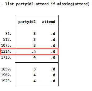
Here, we can see that seven observations were dropped (we do not include "1214" because it does not have a valid entry for partyid2). These seven observations account for in the total number of observations in "partyid2" (1,906) and the number used in the crosstabulation above (1,899).

Handy Tricks

This page covers a few odds and ends that can be helpful at times.

Using the "if" command

Let's say you want to analyze only a subset of the data. For example, let's say you're still interested in what affects attitudes toward federal spending on science and technology, but you want to look specifically at women's attitudes, not men's. You can use the "if" command to subset the data accordingly. So, for a crosstab of science and party id, you would type

tab science partyid if female==1

For a regression of science on partyid, you would type

reg science partyid if female==1

The output is only a regression examining the relationship between partyid and science among female respondents. It's important to note that it takes two equals signs.

Additional model fit statistics

After you run a regression, you can simply type "fitstat" and hit enter to get a wide range of additional model fit statistics. 

For example, think back to the bivariate and multivariate OLS regressions from the last page. How might you decide whether the model with only partyid is better, or if the model with partyid, female, highschool, and collegedegree is better? The AIC value -- AIC stands for the Akaike Information Criterion -- can give you such an assessment. If adding additional variables to your model nonetheless produces a lower AIC value than the model with fewer variables, you have some statistical justification for the choice. 

Setting "more" off

Often if you tell Stata to do something that involves a lot of output, it will only display a screen worth of it and include a blue link at the bottom that reads "---more---." In order to see everything, you have to keep clicking "---more---." If you would prefer Stata just to spit out the entire result at once, you can tell Stata to do so by turning the "more" option off. Simply run the following command: 

set more off

Now this shouldn't happen -- but it probably sometimes will, because that's just how Stata rolls. 

Loading an Excel spreadsheet into Stata

Often research projects start with a dataset you collect and create using Excel. You can load a dataset from Excel into Stata directly, but the easiest way is simply to copy and paste the dataset into the Data Editor (follow the instructions here and make sure you tell Stata to treat the top row as variable names if you copy that in as well). 

Loading an SPSS, etc., dataset into Stata

Every statistical software has its own quirks, one of which is a unique file format for datasets. Stata uses a .dta extension, while SPSS might use .por. The easiest way to open an SPSS file in Stata is to use a program called Stat/Transfer. This software is unfortunately not widely available on the Barnard campus, but many computer labs at Columbia have it in their Quantiative Apps folder along with Stata. It's simple to use. Just select the dataset and tell Stat/Transfer you want it to become a .dta Stata file. If you don't have access to Stat/Transfer, you can also do this conversion in the open source statistical software R, which can be downloaded for free online. 

For many projects, OLS regression will suffice. However, for more advanced work, different types of dependent variables generally call for different types of regression models. This page presents a very rudimentary overview of some other options. 

Logit and Probit models (for dichotomous dependent variables)

Many outcomes of interest are dichotomous: effectively, the categories fall into something and not-something. For these types of dependent variables, logit and probit regression models are a better fit than OLS models. The Stata commands are simple (instead of starting with "reg," you start with "logit" or "probit"), but the interpretation is a bit different. 

In the vast majority of cases, logit and probit models give substantively similar results. This tutorial proceeds using logit models, but similar logic would apply if you wanted to use probit instead. 

Let's say you're really interested in whether people identify as Democrats or not: that is, you aren't interested in the slight degrees of variation, but only in a dichotomous sense of Democrat/not-Democrat. We can make the party identification variable a Democratic dummy variable and use logistic regression to estimate the effect of the independent variables on this outcome (see the do-file for the generation of the Democratic dummy variable). 

Consider the simple hypothesis that women are more likely to be Democrats. This hypothesis can be tested with logistic regression using the following command: 

logit democrat female

The output looks like this: 

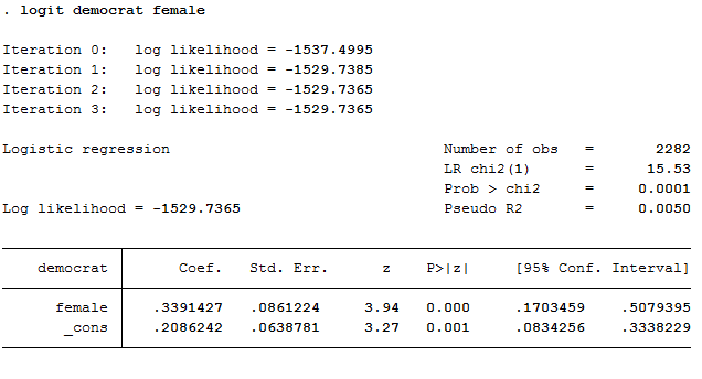
The fact that the coefficient on the independent variable of interest is statistically significant lends some very general credence to our theory, but so far we don't have any real sense of whether the effect is big or small. Looking at marginal effects, rather than the logit coefficients, is one way of making a better assessment of that. 

Calculating marginal effects for Logit and Probit models

Unlike OLS coefficients, Logit and Probit coefficients don't have an intrinsic substantive interpretation attached to them. However, you can easily calculate marginal effects for variables of interest using the "mfx" command. By default, the command calculates the effect holding the other variables at their mean. However, you can manually alter this by adding to the command. In this case, we're just looking at a bivariate model -- there are no other variables besides the one we're focusing on -- so this is sort of beside the point. 

Type the following command after you run your logistic regression: 

mfx

The output looks like this: 

The number under "dy/dx" is the marginal effect of a one-unit shift in the female variable (which is a dummy variable, so that means going from 0 to 1, which means male to female). It turns out women are about 8 percent more likely than men to identify as Democrats. The z-statistic ("z") of 3.94 is greater than 1.96, so this effect is statistically significant at the .05 level. Indeed, as indicated by the 0.000 under "P>|z|," it would be statistically significant even using a more stringent significance level than .05. Our theory is supported by the evidence. 

Ordered Logit/Probit models 

Some outcomes of interest have more than two categories that clearly share an underlying order, but are not quite a scale. An example might be attitudes toward gay marriage: Some people oppose all legal recognition for gay couples. Others support civil unions for gay couples, but not equal access to the traditional institution of marriage. Finally, some people support full equal marriage rights. These three categories can certainly be ordered. The first is the most restrictive, the second is somewhere in between, and the third is the most permissive. Yet it's not necessarily the case that the space between "no legal recognition" and "civil unions only" is the same as the space between "civil unions only" and "full marriage rights." You certainly could use an OLS regression model to estimate such attitudes, but ordered logit and probit models might be more methodologically proper. 

Ordered probit tends to be more commonly used, so we'll use that as our example. But again: the same general logic would apply if you chose to use an ordered logit model instead. 

Let's consider the hypothesis that women are more likely to say they support full marriage rights than just civil unions. Let's also control for party identification and education. After recoding the gay marriage variable a bit (see the do-file for full replication code), I run the following command: 

oprobit gaymarriage female partyid highschool collegedegree

This is the output: 

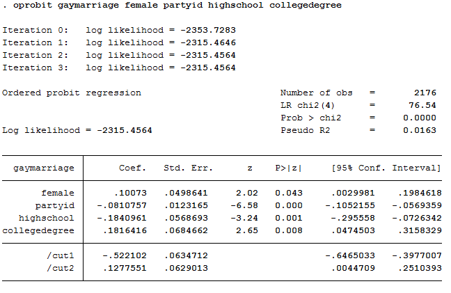
The ordered probit coefficient for the female variable is statistically significant, lending some credence to our theory. However, the number associated with this variable (.10073) doesn't really mean anything substantive. So far all we really know is the relationship is not zero. To get more at the real nature and extent of the effect, you can calculate changes in probabilities.

Calculating changes in probabilities 

You can easily calculate changes in probabilties using the "prchange" command. This command is part of a software package called SPost, which you can download here. You need to install this package before the "prchange" command will run. You can find various ways of doing that on the website, or you can just type:

net install spost9_ado

This provides a simple installation of a slightly older version, which will likely be fine for your purposes (this method assumes you are connected to the internet). After you run your ordered probit model, simply type this command to get changes in probabilities: 

prchange

This gives you the following output: 

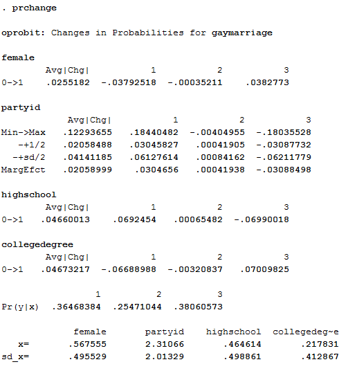
Focus on the numbers immediately below the word female. This tells you the average change associated with this variable is about a three percent shift in probability in the liberal direction. The number under "1" tells you women are about 4 percent less likely to support the first category (no legal recognition) compared to the second category (civil unions only). The number under "2" is basically zero, which suggests women aren't really more or less likely to support civil unions. However, the number under "3" tells you women are about 4 percent more likely to be in the third category (full marriage rights), relative to the second category (civil unions only). Although 4 percentage points is not a huge change, it is consistent with our hypothesis. 

Multinomial logit models

Another potential outcome of interest is one where there are more than two categories, but no clear underlying order. An example might be a question asking respondents what they think the most important problem facing the country is. Answers might include unemployment, the war in Afghanistan, the legality of abortion, balancing the budget, or any other political issue. What makes this type of variable different is that its mulitple categories don't share any underlying order: Unemployment isn't "more" or "less" than the war in Afghanistan, which in turn isn't "more" or "less" than the legality of abortion, and so on. A multinomial logit model would be a better fit for this type of dependent variable, although the assumptions behind multinomial logit models are a bit more involved. The Stata command is "mlogit" and follows the same logic as every other regression command (i.e., if your dependent variable is mostimportantproblem and your independent variables are gender and partyid, your command would be "mlogit mostimportantproblem gender partyid"). However, if you aren't familiar with multinomial logistic regression models, you should be sure to read about how they work before just running the commands. 

This section is still under construction. Need help? Come to the ERL or email us!

Histograms

You can also create a histogram for the variable using the "hist" command by typing: 

hist V083098x

The result of this command is the following: 

This section is still under construction. Need help? Come to the ERL or email us!

Type mismatch

Sometimes the variables you want to use for analysis are of different types and Stata won't allow them to be used together. For example, you might have a string varaible but need it to be a numeric variable. In this case, the "encode" command will usually solve your problem. Simply type "encode variable, gen(variable2)," where "variable" is the name of the string variable you want to convert and "variable2" is the name you're giving the newly converted numeric variable. Be sure to tab out the new variable. If your variable has 5-categories, for instance, encoded variables automatically label the first category 1, the second 2, etc. This can be confusing if the variable originally had a different underlying coding, but it's pretty straight-forward if you're careful about it. 

Not enough space to load a dataset

New versions of Stata automatically allot a sufficient amount of space, but sometimes older versions have trouble loading large datasets. In this case, you can tell Stata to use more memory by typing "set mem 500m" ("500m" is an example; you can pick any value sufficiently large -- but not too large that it slows down your computer!). However, if you try to do this in Stata 12, you will get this message: "Me